5 The importance of collaboration in Bayesian analyses with small samples
Abstract
This chapter addresses Bayesian estimation with (weakly) informative priors as a solution for small sample size issues. Special attention is paid to the problems that may arise in the analysis process, showing that Bayesian estimation should not be considered a quick solution for small sample size problems in complex models. The analysis steps are described and illustrated with an empirical example for which the planned analysis goes awry. Several solutions are presented for the problems that arise, and the chapter shows that different solutions can result in different posterior summaries and substantive conclusions. Therefore, statistical solutions should always be evaluated in the context of the substantive research question. This emphasizes the need for a constant interaction and collaboration between applied researchers and statisticians.
5.1 Introduction
Complex statistical models, such as Structural Equation Models (SEMs), generally require large sample sizes (Tabachnick, Fidell, & Ullman, 2007; Wang & Wang, 2012). In practice, a large enough sample cannot always be easily obtained. Still, some research questions can only be answered with complex statistical models. Fortunately, solutions exist to overcome estimation issues with small sample sizes for complex models, see Smid, McNeish, Miočević, & van de Schoot (2020) for a systematic review comparing frequentist and Bayesian approaches . The current chapter addresses one of these solutions, namely Bayesian estimation with informative priors. In the process of Bayesian estimation, the WAMBS-checklist (When-to-Worry-and-How-to-Avoid-the-Misuse-of-Bayesian-Statistics; Depaoli & van de Schoot, 2017) is a helpful tool; see also van de Schoot, Veen, Smeets, Winter, & Depaoli (2020). However, problems may arise in Bayesian analyses with informative priors, and whereas these problems are generally recognized in the field, they are not always described or solved in existing tutorials, statistical handbooks or example papers. This chapter offers an example of issues arising in the estimation of a Latent Growth Model (LGM) with a distal outcome using Bayesian methods with informative priors and a small data set of young children with burn injuries and their mothers. Moreover, we introduce two additional tools for diagnosing estimation issues: divergent transitions and the effective sample size of the posterior parameter samples, available in Stan (Stan Development Team, 2018b) which makes use of an advanced Hamiltonian Monte Carlo (HMC) algorithm called the No-U-Turn-Sampler (NUTS: Hoffman & Gelman, 2014). These diagnostics can be used in addition to the checks described in the WAMBS checklist.
In the following sections, we briefly introduce LGMs and address the role of sample size, followed by an empirical example for which we present an analysis plan. Next, we show the process of adjusting the analysis in response to estimation problems. We show that different solutions can differentially impact the posterior summaries and substantive conclusions. This chapter highlights the importance of collaboration between substantive experts and statisticians when an initial analysis plan goes awry.
5.2 Latent Growth Models with small sample sizes
Latent Growth Models (LGMs) include repeated measurements of observed variables, and allow researchers to examine change over time in the construct of interest. LGMs can be extended to include distal outcomes and covariates (see Figure 5.1). One of the benefits of specifying an LGM as a structural equation model (SEM), as opposed to a multilevel model as discussed in Hox & McNeish (2020), is that growth can be specified as a non-monotonic or even non-linear function. For instance, we can specify an LGM in which part of the growth process is fixed and another part is estimated from the data. In Figure 5.1, two constraints on the relationships between the latent slope and measurement occasions are freed for two waves, thereby estimating \(\lambda_{22}\) and \(\lambda_{23}\) from the data. As a result, we allow individuals to differ in the way their manifest variables change from the first to the last measurement.
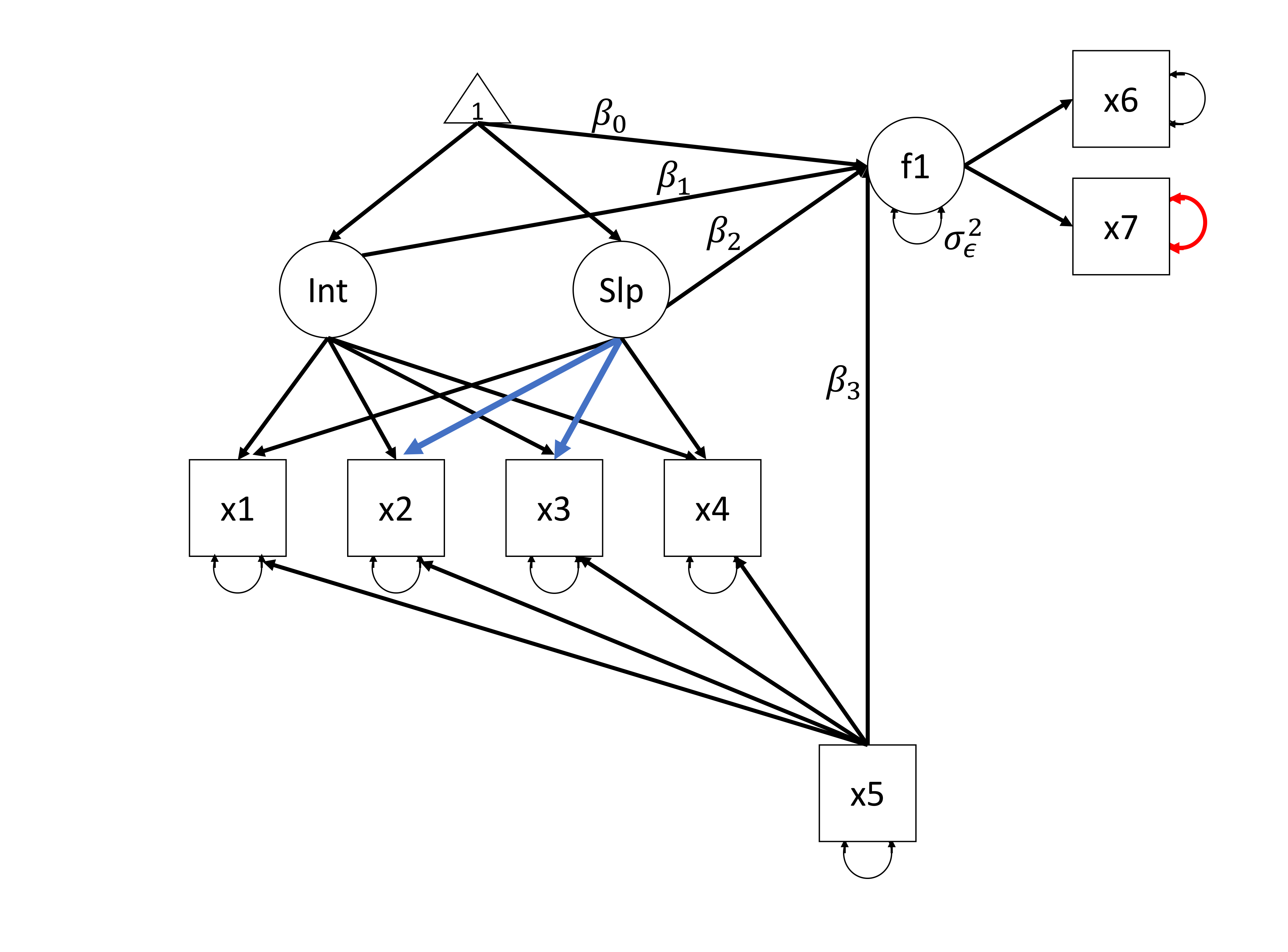
Figure 5.1: The Latent Growth Model as used in the empirical example. The parameters of interest are the intercept of the latent factor f1 (\(\beta_0\)), f1 regressed on the latent intercept (\(\beta_1\)), the latent slope (\(\beta_2\)) and x5 (\(\beta_3\)) and the residual variance of the latent factor f1 (\(\sigma_\epsilon^2\)). The two blue factor loadings indicate freely estimated relationships for \(\lambda_{22}\) and \(\lambda_{23}\) (respectively). The red residual variance parameter (\(\theta_{77}\)) is highlighted throughout the empirical example.
One drawback of LGMs, however, is that such models generally require large sample sizes. The more restrictions we place on a model, the fewer parameters there are to estimate, and the smaller the required sample size. The restrictions placed should, however, be in line with theory and research questions. Small sample sizes can cause problems such as high bias and low coverage (Hox & Maas, 2001), nonconvergence or improper solutions such as negative variance estimates (Wang & Wang, 2012, Chapter 7), and the question is how large should the sample size be to avoid these issues. Several simulation studies using maximum likelihood estimation have provided information on required sample sizes for SEM in general, and LGM specifically. To get an indication of the required sample size, we can use some rather arbitrary rules of thumb. Anderson & Gerbing (1988) recommend N = 100-150 for SEM in general. Hertzog, Oertzen, Ghisletta, & Lindenberger (2008) investigated the power of LGM to detect individual differences in rate of change (i.e., the variance of the latent slope in LGMs). This is relevant for the model in Figure 5.1 because the detection of these differences is needed if the individual rate of change over time (individual parameter estimates for the latent slope) is suitable to be used as a predictor in a regression analysis. In favorable simulation conditions (high Growth Curve Reliability, high correlation between intercept and slope, and many measurement occasions), maximum likelihood estimation has sufficient power to detect individual differences in change with N = 100. However, in unfavorable conditions even a sample size of 500 did not result in enough power to detect individual differences in change. Additionally, the model in the simulation studies by Hertzog and colleagues contained fewer parameters when compared to the LGM model used in the current chapter, thus suggesting that running the model in this chapter would require even larger sample sizes than those recommended by Hertzog and colleagues.
Bayesian estimation is often suggested as a solution for problems encountered in SEM with small sample sizes because it does not rely on the central limit theorem. A recent review examined the performance of Bayesian estimation in comparison to frequentist estimation methods for SEM in small samples on the basis of previously published simulation studies (Smid et al., 2020). It was concluded that Bayesian estimation could be regarded as a valid solution for small sample problems in terms of reducing bias and increasing coverage only when thoughtful priors were specified. In general, naive (i.e., flat or uninformative) priors resulted in high levels of bias. These findings highlight the importance of thoughtfully including prior information when using Bayesian estimation in the context of small samples. Specific simulation studies for LGMs can be found in papers by (McNeish, 2016a, 2016b; Smid, Depaoli, & van de Schoot, 2019; van de Schoot, Broere, Perryck, Zondervan-Zwijnenburg, & van Loey, 2015; Zondervan-Zwijnenburg, Depaoli, Peeters, & van de Schoot, 2018).
In general, it is difficult to label a sample size as small or large, and this can only be done with respect to the complexity of the model. In the remainder of this chapter we use the example of the extensive and quite complex LGM that can be seen in Figure 5.1. We show that with a sample that is small with respect to the complexity of this model, issues arise in the estimation process even with Bayesian estimation with thoughtful priors. Moreover, we provide details on diagnostics, debugging of the analysis and the search for appropriate solutions. We show the need for both statistical and content expertise to make the most of a complicated situation.
5.3 Empirical example: Analysis plan
In practice, there are instances in which only small sample data are available, for example in the case of specific and naturally small or difficult to access populations. In these cases, collecting more data is not an option, and simplifying research questions and statistical models is also undesirable because this will not lead to an appropriate answer to the intended research questions. In this section we introduce an empirical example for which only a small data set was available, and at the same time the research question required the complicated model in Figure 5.1.
5.3.1 Research question, model specification and an overview of data
The empirical example comprises a longitudinal study of child and parental adjustment after a pediatric burn event. Pediatric burn injuries can have long-term consequences for the child’s health-related quality of life (HRQL), in terms of physical, psychological and social functioning. In addition, a pediatric burn injury is a potentially traumatic event for parents, and parents may experience posttraumatic stress symptoms (PTSS; i.e., symptoms of re-experiencing, avoidance and arousal) as a result. Parents’ PTSS could also impact the child’s long-term HRQL. It is important to know whether the initial level of parental PTSS after the event or the development of symptoms is a better predictor of long-term child HRQL, since this may provide information about the appropriate timing of potential interventions. Therefore, the research question of interest was how the initial level and the development of mothers’ posttraumatic stress symptoms (PTSS) over time predict the child’s long-term health-related quality of life (HRQL).
In terms of statistical modelling, the research question required an LGM to model PTSS development and a measurement model for the distal outcome, namely, the child’s HRQL. The full hypothesized model and the main parameters of interest, i.e. the regression coefficients of the predictors for the child’s HRQL, \(\beta_0\) for the intercept, \(\beta_1\) for HRQL regressed on the latent intercept, \(\beta_2\) for HRQL regressed on the latent slope, \(\beta_3\) for HRQL regressed on the covariate, percentage of Total Body Surface Area (TBSA) burned, and the residual variance \(\sigma_\epsilon^2\), are displayed in Figure 5.1.
Mothers reported on PTSS at four time points (up to 18 months) after the burn injury by filling out the Impact of Event Scale (IES; Horowitz, Wilner, & Alvarez, 1979). The total IES score from each of the four time points was used in the LGM. Eighteen months postburn, mothers completed the Health Outcomes Burn Questionnaire (HOBQ; Kazis et al., 2002), which consists of 10 subscales. Based on a confirmatory factor analysis, these subscales were divided into three factors, i.e., Development, Behavior and Concern factors. For illustrative reasons, we only focus on the Behavior factor in the current chapter which was measured by just two manifest variables. TBSA was used to indicate burn severity; this is the proportion of the body that is affected by second- or third-degree burns and it was used as a covariate. For more detailed information about participant recruitment, procedures, and measurements see (Bakker, van der Heijden, Van Son, & van Loey, 2013).
Data from only 107 families was available. Even though data were collected in multiple burn centers across the Netherlands and Belgium over a prolonged period of time (namely 3 years), obtaining this sample size was already a challenge because of two main reasons. Firstly, the incidence of pediatric burns is relatively low. Yearly, around 160 children between the ages of 0 and 4 years old require hospitalization in a specialized Dutch burn center (van Baar, Vloemans, Beerthuizen, Middelkoop, & Nederlandse Brandwonden Registratie R3, 2015). Secondly, the acute hospitalization period in which families were recruited to participate is extremely stressful. Participating in research in this demanding and emotional phase may be perceived as an additional burden by parents.
Still, we aimed to answer a research question that required the complex statistical model displayed in Figure 5.1. Therefore, we used Bayesian estimation with weakly informative priors to overcome the issues of small sample size estimation with ML-estimation, for which the model shown in Figure 5.1 resulted in negative variance estimates.
5.3.2 Specifying and understanding priors
The specification of the priors is one of the essential elements of Bayesian analysis, especially when the sample size is small. Given the complexity of the LGM model relative to the sample size, prior information was incorporated to facilitate the estimation of the model (i.e., step 1 of the WAMBS-checklist). In addition to careful consideration of the plausible parameter space, we used previous results to inform the priors in our current model (Egberts, van de Schoot, Geenen, & van Loey, 2017).
The prior for the mean of the latent intercept (\(\alpha_1\)) could be regarded as informative with respect to the location specification. The location parameter, or mean of the normally distributed prior \(N(\mu_0, \sigma_0^2)\), was based on the results of a previous study (Egberts et al., 2017, Table 1) and set at 26. If priors are based on information from previously published studies, it is important to reflect on the exchangeability of the prior and current study, see for instance Miočević, Levy, & Savord (2020). Exchangeability would indicate that the samples are drawn from the same population and a higher prior certainty can be used. To evaluate exchangeability, the characteristics of the sample and the data collection procedure were evaluated. Both studies used identical questionnaires and measurement intervals, and the data were collected in exactly the same burn centers. The main difference between the samples was the age of the children (i.e., age range in the current sample: 8 months-4 years; age range in the previous sample: 8-18 years), and related to that, the age of the mothers also differed (i.e., mean age in the current sample: 32 years; mean age in the previous sample: 42 years). Although generally, child age has not been associated with parents’ PTSS after medical trauma (e.g., Landolt, Vollrath, Ribi, Gnehm, & Sennhauser, 2003), the two studies are not completely exchangeable as a results of the age difference. Therefore, additional uncertainty about the value of the parameter was specified by selecting a relatively high prior variance (see Table 5.1).
The priors for the regression coefficients are related to the expected scale of their associated parameters. For \(\beta_1\) a \(N(0,4)\) prior was specified, thereby allocating the most density mass on the plausible parameter space. Therefore, given the scale of the instruments used, and the parametrization of the factor score model, the latent factor scores can take on values between zero and 100. A regression coefficient of -4 or 4 would be extremely implausible. If our expected value of 26 is accurate for the intercept, this would change our predicted factor score by -104 or 104, respectively. This would constitute a change larger than the range of the construct. For \(\beta_2\) in contrast, a \(N(0, 2500)\) prior was specified because small latent slope values, near the prior group mean of the latent slope of zero, should be allowed to have large impacts on the latent factor scores. For instance, a slope value of 0.1 could be associated with a drop of 50 in HRQL, resulting in a coefficient of -500. Figure 5.2 shows what would have happened to the prior predictive distributions for the latent factor scores if a N(0,2500) prior was specified for \(\beta_1\) instead of the \(N(0, 4)\) prior, keeping all other priors constant. The prior predictive densities for the factor scores in panel B of Figure 5.2 place far too much support on parts of the parameter space that are impossible. The factor scores can only take on values between zero and 100 in our model specification. For more information on prior predictive distributions, see for instance van de Schoot et al. (2020).
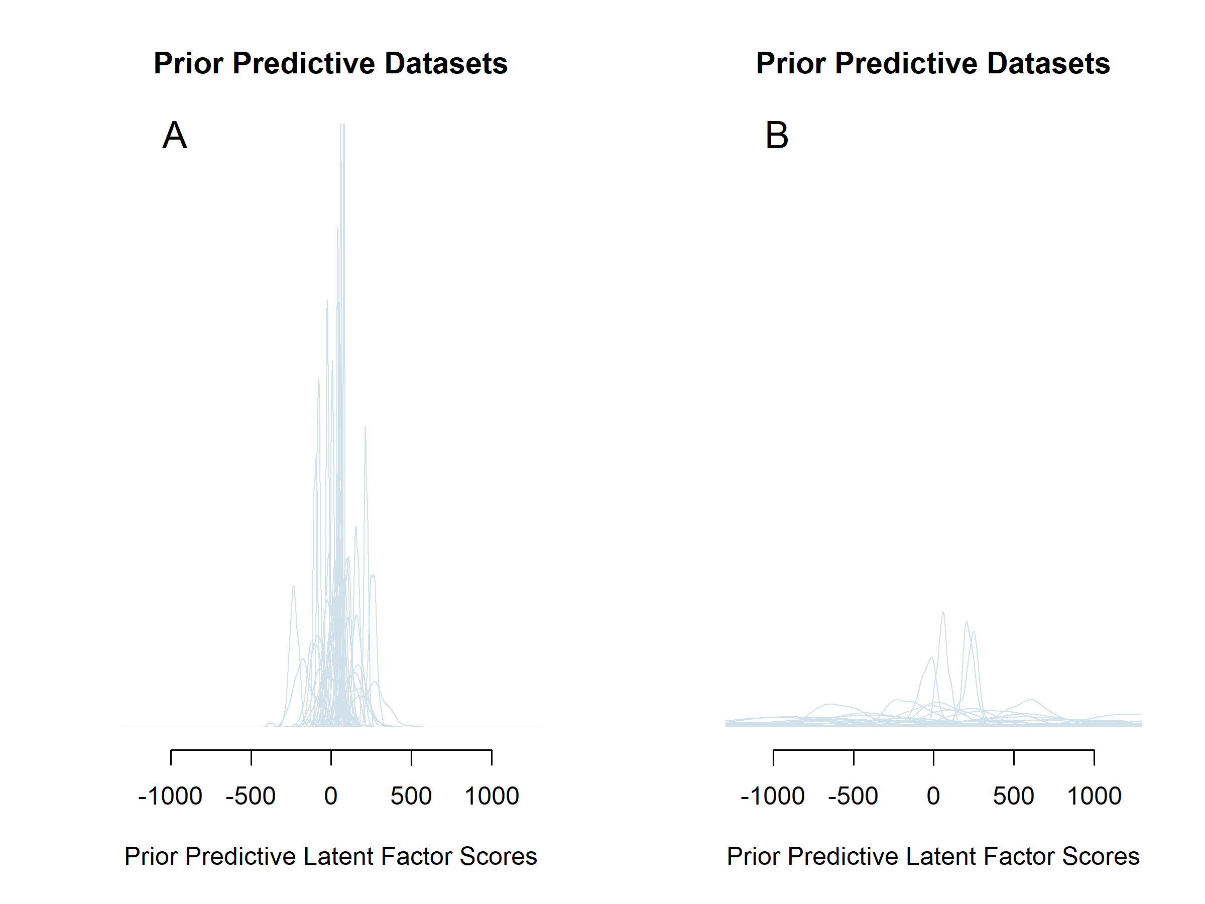
Figure 5.2: The effect of changing a single prior in the model specification on the prior predictive distributions of the Latent Factor Scores. The prior for \(\beta_1\) is changed from weakly informative (panel A; \(N(0,4)\)) to uninformative (panel B; \(N(0,2500)\)).
| Parameter | Prior | Justification |
|---|---|---|
| group mean of the latent intercept (\(\alpha_1\)) | \(N(26, 400)\) | Previous article on different cohort (Egberts et al., 2017, Table 1) |
| group standard deviation of the latent intercept (\(\sigma_{Int}\)) | \(HN(0, 400)\) | Allows values to cover entire parameter space for IES |
| group mean of the latent slope (\(\alpha_2\)) | \(N(0, 4)\) | Allows values to cover entire parameter space for IES |
| group standard deviation of the latent slope (\(\sigma_{slope}\)) | \(HN(0, 1)\) | Allows values to cover entire parameter space for IES |
| \(x1-x4\) regressed on \(x5\) (\(\beta_{ies}\)) | \(N(0, 4)\) | Allows values to cover entire parameter space for IES |
| group mean relation IES 3 months (\(x2\)) regressed on slope (\(\mu_{\lambda_{22}}\)) | \(N(3, 25)\) | Centered at 3 which would be the constraint in a linear LGM. Allowed to vary between individuals to allow for between-person differences in the way manifest variables change from the first to the last measurement |
| group mean relation IES 12 months (\(x3\)) regressed on slope (\(\mu_{\lambda_{23}}\)) | \(N(12, 25)\) | Centered at 12 which would be the constraint in a linear LGM. Allowed to vary between individuals to allow for between-person differences in the way manifest variables change from the first to the last measurement. |
| group standard deviation relation IES 3 months (\(x2\)) regressed on slope (\(\sigma_{\lambda_{22}}\)) | \(HN(0, 6.25)\) | Allows for large and small between-person differences in the way manifest variables change from the first to the last measurement. |
| group standard deviation relation IES 12 months (\(x3\)) regressed on slope (\(\sigma_{\lambda_{23}}\)) | \(HN(0, 6.25)\) | Allows for large and small between-person differences in the way manifest variables change from the first to the last measurement. |
| All residual standard deviations \(x1-x4\) (\(\sigma_{\epsilon_{ies}}\)) | \(HN(0, 100)\) | Allows values to cover entire parameter space for the observed variables |
| Intercepts factor regressions (\(\beta_0\)) | \(N(50, 2500)\) | Covers full factor score parameter space centered at middle |
| Factors regressed on Level (\(\beta_1\)) | \(N(0, 4)\) | Allows values to cover entire parameter space for the factor scores |
| Factors regressed on Shape (\(\beta_2\)) | \(N(0, 2500)\) | Allows values to cover entire parameter space for the factor scores |
| Factors regressed on TBSA (\(\beta_3\)) | \(N(0, 4)\) | Allows values to cover entire parameter space for the factor scores |
| Residual standard deviation factors (\(\sigma_\epsilon\)) | \(HN(0, 100)\) | Allows values to cover entire parameter space for the residuals |
5.4 Empirical example: Conducting the analysis
Based on theoretical considerations, we specified the model as shown in Figure 5.1 using the priors as specified in Table 5.1. We used Stan (Carpenter et al., 2017) via RStan (Stan Development Team, 2018b) to estimate the model and we used the advanced version of the Hamiltonian Monte Carlo (HMC) algorithm called the No-U-Turn sampler (NUTS; Hoffman & Gelman, 2014). To run the model, we used the following code which by default ran the model using four chains with 2000 MCMC iterations of which 1000 are warmup samples:
fit_default <- sampling(model, data = list(X = X, I, K,
                                           run_estimation = 1),
                        seed = 11,  show_messages = TRUE)
For reproducibility purposes, the OSF webpage (https://osf.io/am7pr/) includes all annotated Rstan code and the data.
Upon completion of the estimation, we received the following warnings from Rstan indicating severe issues with the estimation procedure:
Warning messages:
1: There were 676 divergent transitions after warmup.
Increasing adapt_delta above 0.8 may help. See:
http://mc-stan.org/misc/warnings.html#divergent-transitions-after-warmup
2: There were 16 transitions after warmup that exceeded the
maximum treedepth. Increase max_treedepth above 10. See
http://mc-stan.org/misc/warnings.html#maximum-treedepth-exceeded
3: There were 4 chains where the estimated
Bayesian Fraction of Missing Information was low.
See http://mc-stan.org/misc/warnings.html#bfmi-low
4: Examine the pairs() plot to diagnose sampling problems
Fortunately, the warning messages also pointed to online resources with more detailed information about the problems. In what follows, we describe two diagnostics to detect issues in the estimation procedure: divergent transitions (this section) and the effective sample size of the MCMC algorithm (next section).
The most important warning message is about divergent transitions (warning message 1). The appearance of divergent transitions is a strong indicator that the posterior results as shown in column 1 of Table 5.3 cannot be trusted (Stan Development Team, 2019, Chapter 14). For detailed, highly technical information on this diagnostic, see Betancourt (2016). Very loosely formulated, the occurrence of many divergent transitions indicates that there is something going wrong in drawing MCMC samples from the posterior. When the estimator moves from one iteration to the next, it does so using a particular step size. The larger steps the estimator can take between iterations, the more effectively it can explore the parameter space of the posterior distribution (compare Figure 5.3A with 5.3B). When a divergent transition occurs, the step size is too large to efficiently explore part of the posterior distribution and the sampler runs into problems when transitioning from one iteration to the next, (see Figure 5.3C). The Stan Development Team uses the following analogy to provide some intuition for the problem:
“For some intuition, imagine walking down a steep mountain. If you take too big of a step you will fall, but if you can take very tiny steps you might be able to make your way down the mountain, albeit very slowly. Similarly, we can tell Stan to take smaller steps around the posterior distribution, which (in some but not all cases) can help avoid these divergences.”
The posterior results for the parameters of interest (\(\beta_0, \beta_1, \beta_2, \beta_3, \sigma_\epsilon\)) are shown in Table 5.3, column 1. Note that these results cannot be trusted and should not be interpreted because of the many divergent transitions. Divergent transitions can sometimes be resolved by simply taking smaller steps (see next section), which increases computational time.
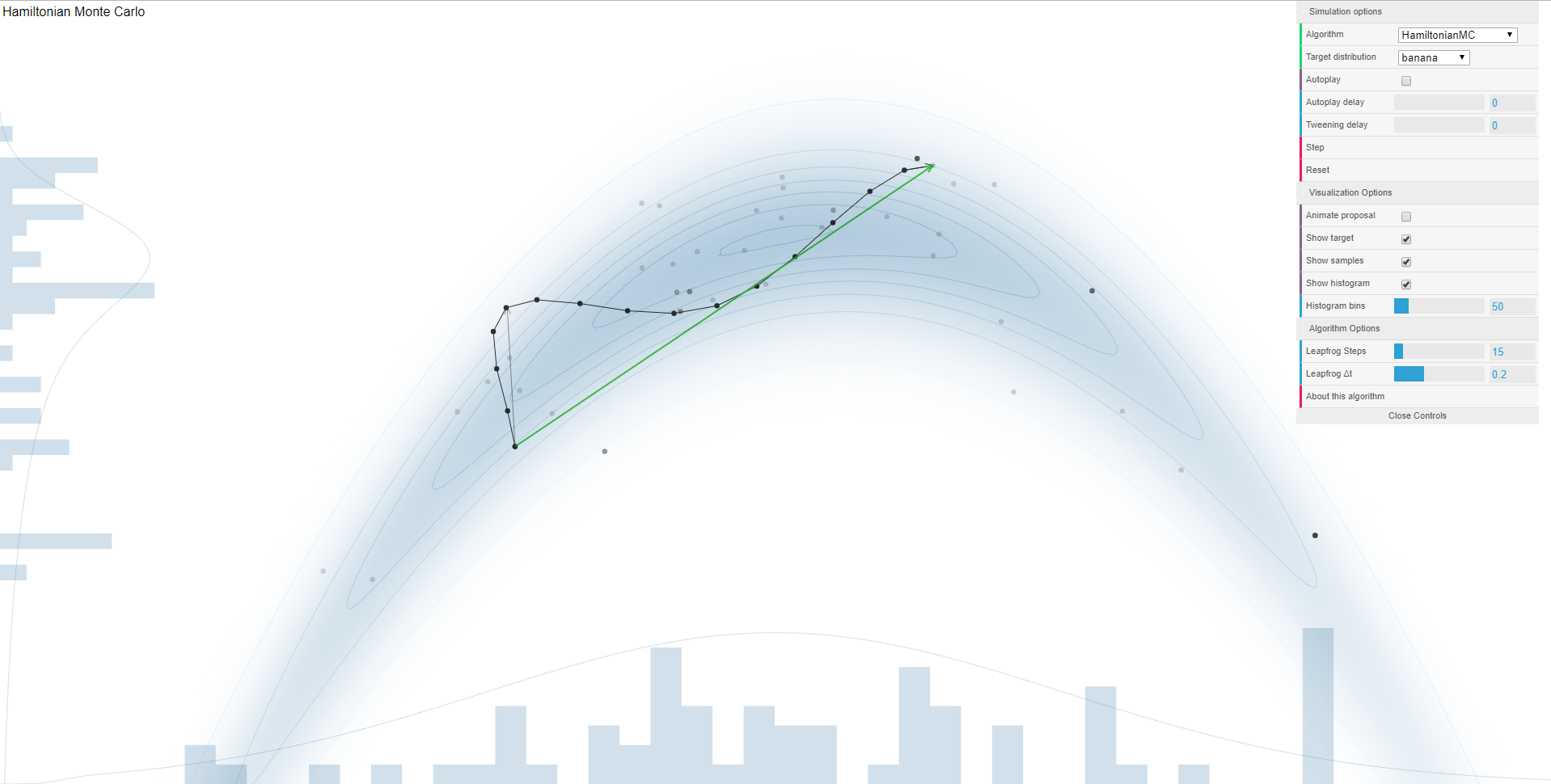
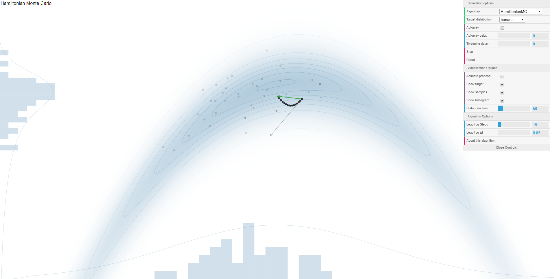
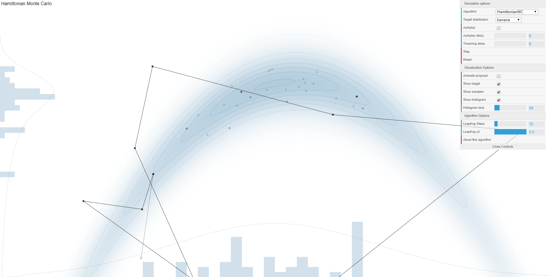
Figure 5.3: Effect of decreasing the step size of the HMC on the efficiency of the exploration of the posterior distribution (Panel A and B). The green arrow shows the step between two consecutive iterations. Panel A uses a large step size and swiftly samples from both posterior distributions, one of which is a normal distribution and one of which a common distributional form for variance parameters. Panel B, in contrast, needs more time to sample from both distributions and describe them accurately because the steps are a lot smaller in between iterations. Panel C shows an example of a divergent transition, which is indicative of problems with the sampling algorithm. These screenshots come from an application developed by Feng (2016) that provides insight into different Bayesian sampling algorithms and their behavior for different shapes of posterior distributions.
5.5 Debugging
The occurrence of divergent transitions can also be an indication of more serious issues with the model or with a specific parameter. One of the ways to find out which parameter might be problematic is to inspect how efficiently the sampler sampled from the posterior of each parameter. The efficiency of the sampling process can be expressed as the Effective Sample Size (ESS) for each parameter, where sample size does not refer to the data but to the samples taken from the posterior. In the default setting we saved 1000 of these samples per chain, so in total we obtained 4000 MCMC samples for each parameter. However, these MCMC samples are related to each other, which can be expressed by the degree of autocorrelation (point 5 on the WAMBS checklist in Chapter 3). ESS expresses how many independent MCMC samples are equivalent to the autocorrelated MCMC samples that were drawn. If a small ESS for a certain parameter is obtained, there is little information available to construct the posterior distribution of that parameter. This will also manifest itself in the form of autocorrelation and non-smooth histograms of posteriors. For more details on ESS and how RStan calculates it, see the Stan Reference Manual (Stan Development Team, 2019).
In Table 5.2 we provide the ESS for \(\alpha_1, \beta_1, \theta_{77}\) and the factor score of mother and child pair no. 33 (denoted by \(fs_{33}\)).\(fs_{33}\) was estimated efficiently and the ESS was 60% of the number of MCMC samples, followed by \(\alpha_1\) (14%) and \(\beta_1\) (11%). \(\theta_{77}\), in contrast, had an ESS of only 0.5% of the number of MCMC samples indicating an equivalence of only 20 MCMC samples had been used to construct the posterior distribution. There is no clear cut-off value for the ESS, although it is obvious that higher values are better and that 20 is very low. The default diagnostic threshold used in the R package shinystan (Gabry, 2018), used for interactive visual and numerical diagnostics, is set to 10%.
The effects of ESS on the histograms of these four parameters can be seen in Figure 5.4 which shows a smooth distribution for \(fs_{33}\) but not for \(\theta_{77}\). Based on the ESS and the inspection of Figure 5.4, the residual variance parameter \(\theta_{77}\) was estimated with the lowest efficiency and probably exhibited the most issues in model estimation.
| Parameter | Model with default estimation settings | Model with small step size in estimation setting | Alternative I: Remove perfect HRQL scores | Alternative II: \(IG(0.5, 0.5)\) prior for \(\theta_{77}\) | Alternative III: Replace factor score with \(x7\) | Alternative IV: Possible increase of variance in latent factor |
|---|---|---|---|---|---|---|
| \(fs_{33}\) | 2390 (60%) | 9843 (123%) | 2219 (55%) | 1307 (33%) | - | 2485 (62%) |
| \(\alpha_1\) | 575 (14%) | 1000 (13%) | 655 (16%) | 145 (4%) | 227 (6%) | 611 (15%) |
| \(\beta_1\) | 424 (11%) | 1966 (25%) | 487 (12%) | 647 (16%) | 58 (1%) | 1004 (25%) |
| \(\theta_{77}\) | 20 (0.5%) | 12 (0.2%) | 9 (0.2%) | 33 (0.8%) | - | 46 (1.2%) |
To investigate if there were systematic patterns in the divergences, we plotted the samples of the parameters \(fs_{33}\) and \(\theta_{77}\) against the log posterior (denoted by \(lp\)) (see Figure 5.5). \(lp\) is, very loosely formulated, an indication of the likelihood of the data given all posterior parameters. \(lp\) is sampled for each MCMC iteration as just another parameter. Note that, in contrast to log-likelihoods, \(lp\) cannot be used for model comparison. Plots such as those in Figure 5.5 can point us to systematic patterns for the divergent transitions, which would indicate that a particular part of the parameter space is hard to explore. In Figure 5.5A it can be seen that for \(fs_{33}\), which did not exhibit problems in terms of ESS, the divergent transitions are more or less randomly distributed across the posterior parameter space. Also, the traceplot and histogram for \(fs_{33}\) would pass the WAMBS-checklist on initial inspection. There is one hotspot around the value of -1700 for the \(lp\) where a cluster of divergent transitions occurs. This is also visible in the traceplot, where it can be seen that one of the chains is stuck and fails to efficiently explore the parameter space shown as an almost horizontal line for many iterations. On closer inspection, a similar behavior in one of the chains could be seen for \(fs_{33}\) as well.
In Figure 5.5B it can be seen that for \(\theta_{77}\), which exhibited problems in terms of ESS, the divergent transitions occur mainly in a very specific part of the posterior parameter space, i.e., many divergent transitions occur close to zero. This also shows up in the traceplot, where for several iterations the sampler could not move away from zero. This indicates that our sampling algorithm ran into problems when exploring the possibility that \(\theta_{77}\) might be near zero. Note that a similar issue arises in one chain around the value of 2.5 for many iterations, resulting in a hot spot which corresponds to the deviant chain for \(lp\). Perhaps an additional parameter could be found which explains the issues concerning this systematic pattern of divergent transitions. For now, we continued with a focus on \(\theta_{77}\).
The first solution, also offered in the warning message provided by Stan, was to force Stan to use a smaller step size by increasing the adapt_delta setting of the estimator. We also deal with the second warning by increasing max_treedepth, although this is related to efficiency and not an indication of model error and validity issues. To make sure we could still explore the entire posterior parameter space, we extended the number of iterations post warmup to 2000 for each chain (iter – warmup in the code below). We used the following R code:
fit_small_step <- sampling(model,
                           data=list(X = X, I, K, run_estimation = 1),
                           control=list(adapt_delta = .995,
                                        max_treedepth = 16),
                           warmup = 3000, iter = 5000, seed = 11235813)
We inspected the ESS for the same parameters again, which can be seen in Table 5.2. The problems seem to occur for the \(\theta_{77}\) parameter again, and it has even decreased in efficiency. We compared the posterior for \(\theta_{77}\) and \(lp\) between the default estimation settings and the estimation settings forcing a smaller step size in Figure 5.6. The smaller step sizes have decreased the number of divergent transitions to almost zero. Also, they enabled more exploration of posterior parameter values near zero. However, the posterior distribution still showed signs of problematic exploration given the strange pattern of MCMC samples close to 0.5 (see step 6 of the WAMBS checklist; do posterior estimates make substantive sense?). Apparently, the solution offered by the Rstan warning message to decrease the step size, which often solves the issue of obtaining divergent transitions, failed to provide an efficient result in this case. Thus the posterior estimates in Table 5.3, column 2 still cannot be trusted. In the next section, we briefly explore different solutions that might help us to obtain trustworthy results.
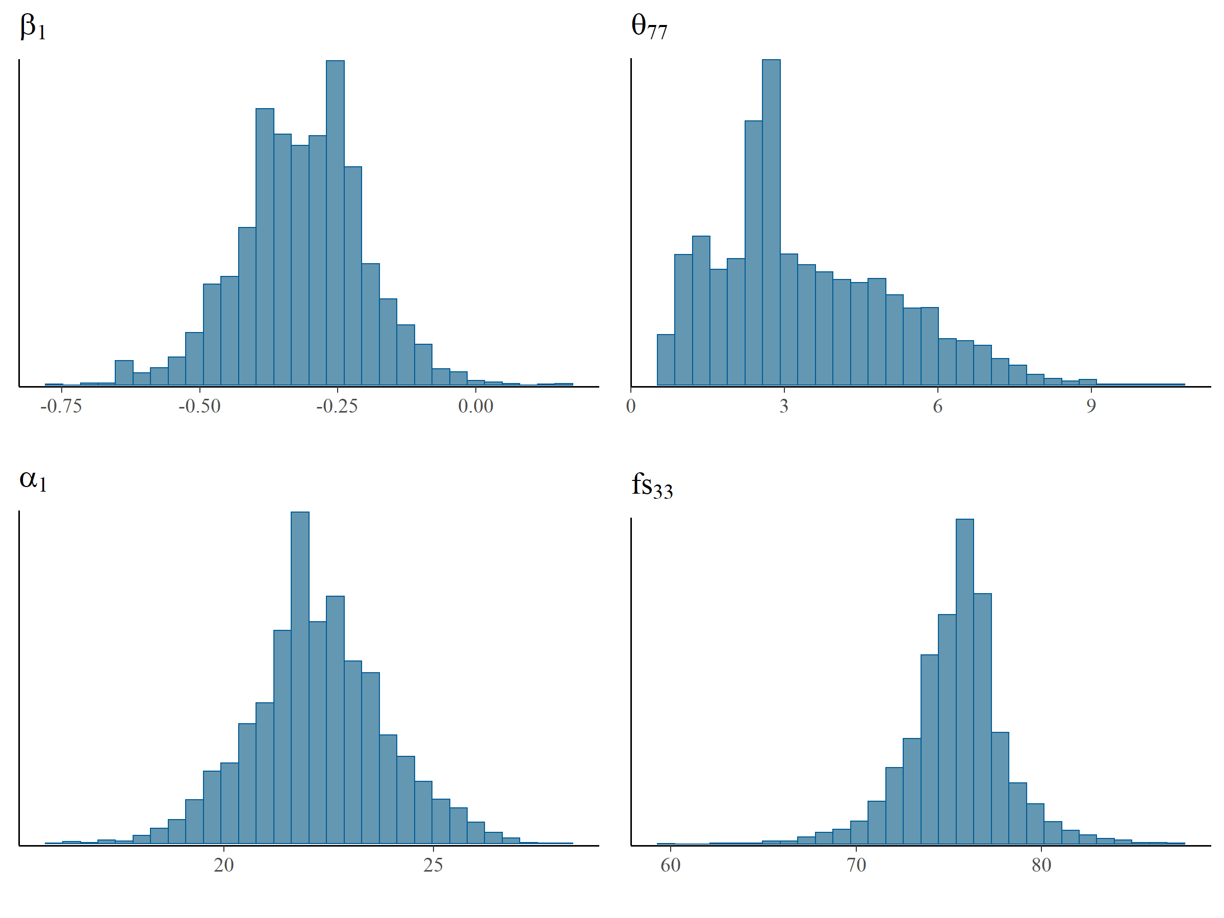
Figure 5.4: Histograms of MCMC samples for \(\alpha_1, \beta_1, \theta_{77}\) and \(fs_{33}\). \(\theta_{77}\) has a non-smooth histogram, which indicates low ESS while the smooth histogram for \(fs_{33}\) is indicative of higher ESS.
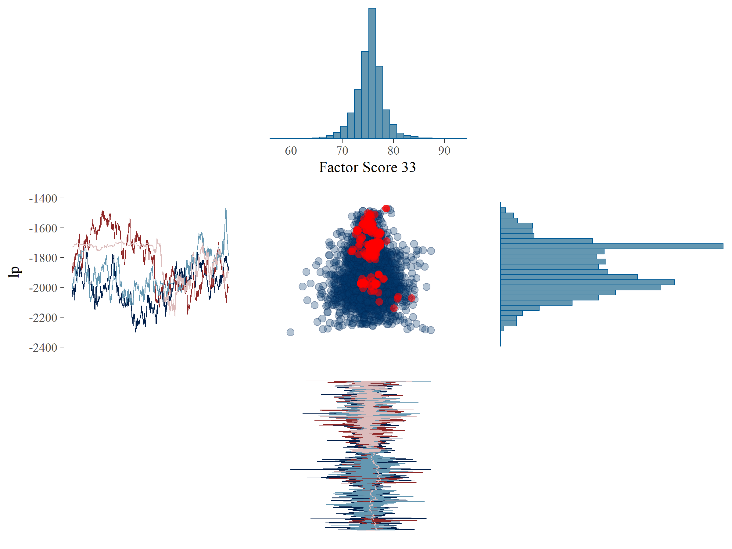
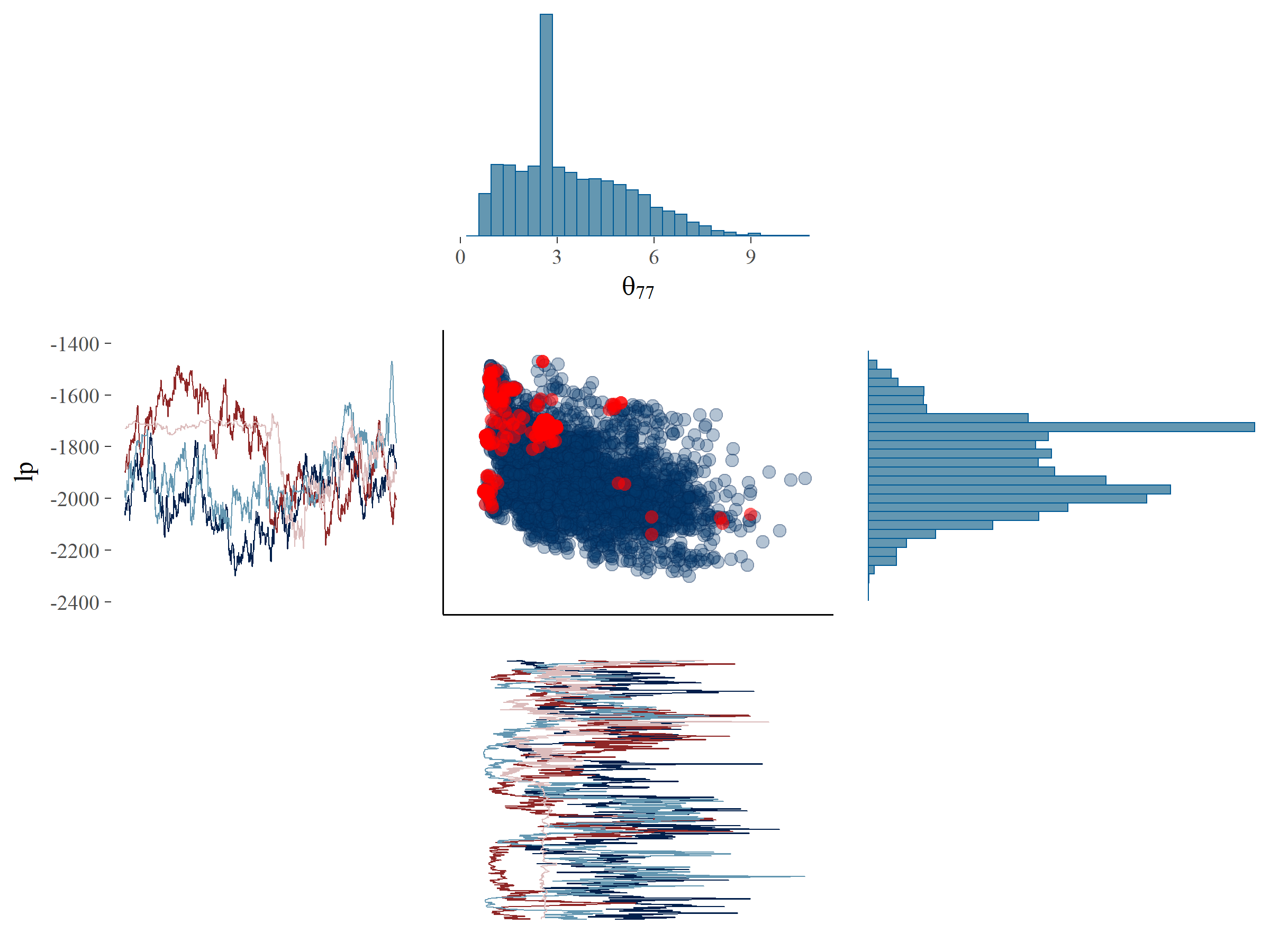
Figure 5.5: Plot of the posterior samples of \(lp\) (y-axis) against \(fs_{33}\) (x-axis, panel A) and \(\theta_{77}\) (x-axis, panel B) with divergent transitions marked by red dots. Additionally, the histograms and trace plots of the corresponding parameters have been placed on the margins.
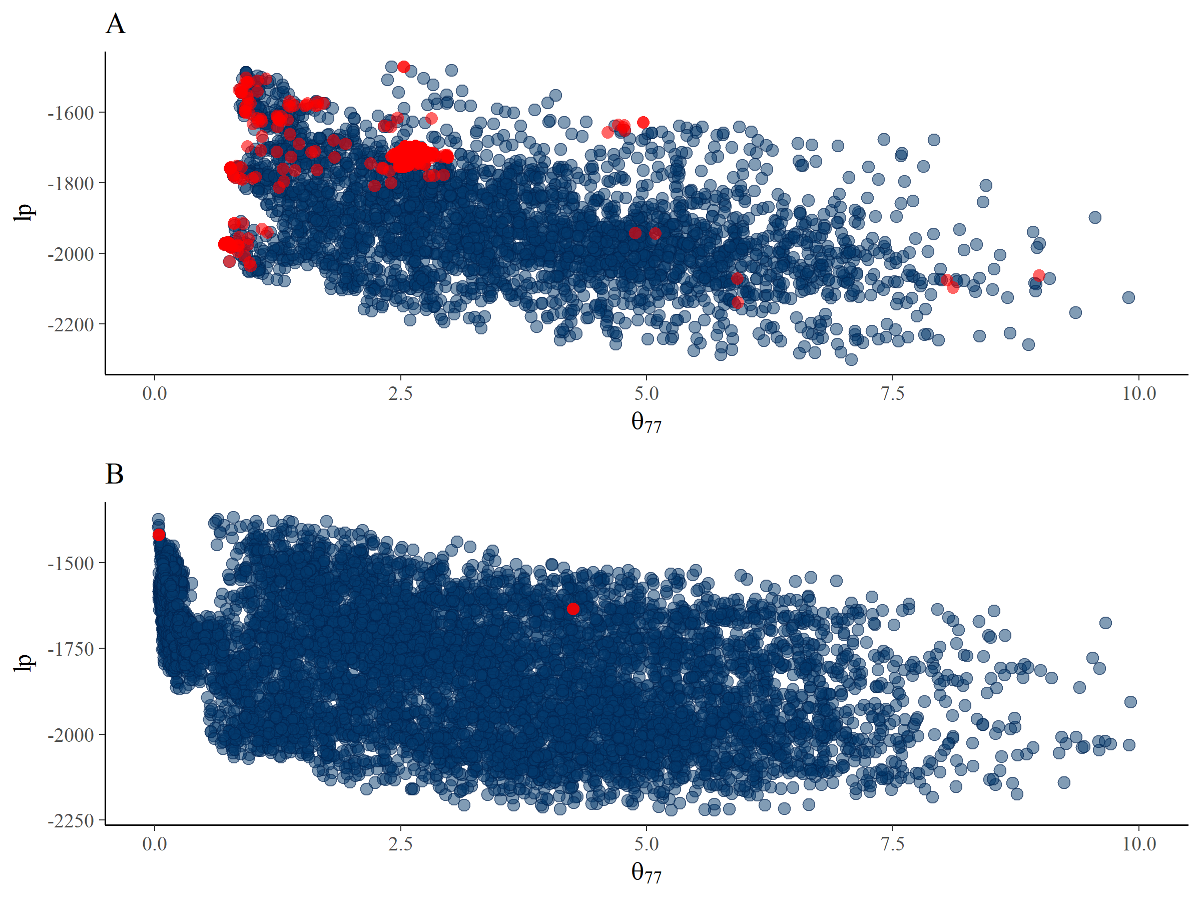
Figure 5.6: Plots of the posterior samples of \(lp\) against \(\theta_{77}\) for the default estimation settings (panel A) and the estimation settings that have been forced to take smaller step sizes (panel B). Divergent transitions are indicated by red dots.
5.6 Moving forward: Alternative Models
At this stage in the analysis process we continue to face difficulties with obtaining trustworthy posterior estimates due to divergent transitions. After exploring a smaller step size in the previous section, there are multiple options that can be considered and these can be based on statistical arguments, substantive theoretical arguments or, ideally, on both. Some statistical options can be sought in terms of the reparameterization of the model (Gelman, 2004), that is, the reformulation of the same model in an alternative form, for instance by using non-centered parametrizations in hierarchical models (Betancourt & Girolami, 2015). This needs to be done carefully and with consideration of the effects on prior implications and posterior estimates. The optimal course of action will differ from one situation to another, and we show five arbitrary ways of moving forward, but all require adjustments to the original analysis plan. We considered the following options: 1. Subgroup removal: We removed 32 cases that scored perfectly, i.e. a score of 100, on the manifest variable \(x7\). This would potentially solve issues with the residual variance of \(x7\) (\(\theta_{77}\)). 2. Changing one of the priors: We specified a different prior on \(\theta_{77}\), namely, an Inverse Gamma (\(IG(0.5,0.5)\)) instead of a Half-Normal (\(HN(0,100)\)) (see: van de Schoot et al., 2015). The IG prior forced the posterior distribution away from zero. If \(\theta_{77}\) was zero, this implies that \(x7\) is a perfect indicator of the latent variable. Since a perfect indicator is unlikely, we specified a prior that excludes this possibility. 3. Changing the distal outcome: We replaced the latent distal outcome with the manifest variable \(x7\). \(\theta_{77}\) estimates contained values of zero, which would indicate that x7 is a good or perfect indicator and could serve as a proxy for the latent variable. Replacing the latent factor with a single manifest indicator reduces the complexity of the model. 4. A possible increase of variance in the distal latent factor score: we removed cases that exhibited little variation between the scores on \(x6\) and \(x7\).
We ran the model using these four adjustments (see the OSF webpage for details). Table 5.3 presents the posterior results of these additional analyses and an assessment of the extent to which the alternatives required adjustments to the original research question. The first three alternative solutions still contained divergent transitions and consequently the results could not be trusted. The fourth alternative solution did not result in divergent transitions. The ESS of the fourth alternative solution was still low, both in terms of the percentage of iterations and in absolute value (see Table 5.2). Although the low ESS in terms of percentage may not be resolved, the absolute ESS can be raised by increasing the total number of iterations. Even though we could draw conclusions using results from the fourth alternative solution, the rather arbitrary removal of cases changed the original research question. We investigated, and thus generalized to, a different population compared to the original analysis plan. Using an alternative model or a subset of the data could provide a solution to estimation issues. However, this could impact our substantive conclusions, e.g., see \(\beta_1\) in Table 5.3, for which the 95% credibility interval in the fourth alternative contained zero, in contrast to credibility intervals for this parameter obtained using other alternative solutions. As substantive conclusions can be impacted by the choices we make, the transparency of the research process is crucial.
| Parameter | Model with default estimation settings | Model with small step size in estimation setting | Alternative I: Remove perfect HRQL scores | Alternative II: \(IG(0.5, 0.5)\) prior for \(\theta_{77}\) | Alternative III: Replace factor score with \(x7\) | Alternative IV: Possible increase of variance in latent factor |
|---|---|---|---|---|---|---|
| \(\beta_0\) | 66.28 [39.58, 83.68] | 66.83 [38.89, 84.12] | 65.56 [48,78, 75.83] | 62.10 [30.95, 83.52] | 69.76 [39.04, 93.51] | 64.46 [47.21, 78.71] |
| \(\beta_1\) | -0.32 [-0.55, -0.10] | -0.31 [-0.53, -0.09] | -0.23 [-0.44, -0.01] | -0.32 [-0.53, -0.10] | -0.40 [-0.67, -0.11] | -0.22 [-0.51, 0.10] |
| \(\beta_2\) | -31.87 [-74.80, -7.63] | -31.46 [-76.41, -7.42] | -19.39 [-44.93, -7.47] | -39.16 [-92,18,-7.81 | -47.06 ] [-96.94, -12 | -35.66 .19] [-64.16, -15.30] |
| \(\beta_3\) | -0.61 [-0.92, -0.31] | -0.62 [-0.93, -0.31] | -0.40 [-0.67, -0.14] | -0,61 [-0,93, -0,30] | -0.78 [-1.16, -0.41] | -0.53 [-1.02, -0.06] |
| \(\sigma_\epsilon\) | 8.36 [3.77, 10.88] | 7.93 [2.92, 10.77] | 4.76 [0.54, 8.29] | 7.40 [1.98, 10.87] | 10.06 [3.73, 13.74] | 6.63 [2.07, 10.63] |
| Divergent transitions present | YES | YES | YES | YES | YES | NO |
| To what extent do we need to adjust analytic strategy? | Not at all | Not at all | Substantially; we generalize to a different (known) population. | Negligible; theory behind research question remains the same. | Substantially; data-driven change of model (replacing measurement model with a single manifest variable). | Substantially; we generalize to a different (unknown) population. |
5.7 Conclusion
Bayesian estimation with (weakly) informative priors is suggested as a solution to deal with small sample size issues. The current chapter illustrated the process of conducting Bayesian estimation with (weakly) informative priors along with the potential problems that can arise. The WAMBS-checklist was a helpful tool in this process, and we propose supplementing the checklist steps with an inspection of the effective number of samples taken using MCMC. As we have shown, a low ESS can point toward specific parameters to investigate, which is especially useful for complex models with many parameters, as investigating each parameter individually would be time-consuming. We recommend using advanced statistical software (such as stan) because the implemented algorithms (e.g., HMC or NUTS) can have a positive impact on the ESS, and estimates of ESS are readily available. Moreover, the use of advanced algorithms such as HMC or NUTS provides additional diagnostic information about the estimation in the form of divergent transitions, which can be used in addition to the WAMBS-checklist.
The empirical example showed that even Bayesian estimation with informative priors has limits in terms of its performance for complex models with small sample sizes. Thus, using a Bayesian analysis should not be considered a ‘quick fix’. Careful consideration of the analysis steps and the intermediate results is imperative. Different solutions can differentially impact the posterior parameter estimates and thereby the substantive conclusions, and there is a need for constant interaction and collaboration between applied researchers, who formulate the research questions, and the statisticians, who possess the statistical and methodological knowledge.
5.8 Acknowledgements
Both authors were supported by the Netherlands Organization for Scientific Research (grant number NWO-VIDI-452-14-006). This work was a result of the collaborative efforts of our project team, including Dr. Nancy van Loey and prof. Dr. Rens van de Schoot. The synthetic data used in the empirical example were based on a study funded by the Dutch Burns Foundation (Grant No. 07.107). We thank all participating parents and the research team in the burn centers in the Netherlands and Belgium.
References
Anderson, J. C., & Gerbing, D. W. (1988). Structural equation modeling in practice: A review and recommended two-step approach. Psychological Bulletin, 103(3), 411.
Bakker, A., van der Heijden, P. G., Van Son, M. J., & van Loey, N. E. (2013). Course of traumatic stress reactions in couples after a burn event to their young child. Health Psychology, 32(10), 1076.
Betancourt, M. (2016). Diagnosing Suboptimal Cotangent Disintegrations in Hamiltonian Monte Carlo. arXiv Preprint arXiv:1604.00695.
Betancourt, M., & Girolami, M. (2015). Hamiltonian Monte Carlo for hierarchical models. Current Trends in Bayesian Methodology with Applications, 79, 30.
Carpenter, B., Gelman, A., Hoffman, M. D., Lee, D., Goodrich, B., Betancourt, M., … Riddell, A. (2017). Stan: A probabilistic programming language. Journal of Statistical Software, 76(1).
Depaoli, S., & van de Schoot, R. (2017). Improving transparency and replication in Bayesian statistics: The WAMBS-Checklist. Psychological Methods, 22(2), 240.
Egberts, M. R., van de Schoot, R., Geenen, R., & van Loey, N. E. (2017). Parents’ posttraumatic stress after burns in their school-aged child: A prospective study. Health Psychology, 36(5), 419.
Feng, C. (2016). The Markov-chain Monte Carlo Interactive Gallery. Retrieved from https://chi-feng.github.io/mcmc-demo/
Gabry, J. (2018). Shinystan: Interactive Visual and Numerical Diagnostics and Posterior Analysis for Bayesian Models. Retrieved from https://CRAN.R-project.org/package=shinystan
Gelman, A. (2004). Parameterization and Bayesian modeling. Journal of the American Statistical Association, 99(466), 537–545.
Hertzog, C., Oertzen, T. von, Ghisletta, P., & Lindenberger, U. (2008). Evaluating the power of latent growth curve models to detect individual differences in change. Structural Equation Modeling: A Multidisciplinary Journal, 15(4), 541–563.
Hoffman, M. D., & Gelman, A. (2014). The No-U-Turn sampler: Adaptively setting path lengths in Hamiltonian Monte Carlo. Journal of Machine Learning Research, 15(1), 1593–1623.
Horowitz, M., Wilner, N., & Alvarez, W. (1979). Impact of Event Scale: A measure of subjective stress. Psychosomatic Medicine, 41(3), 209–218.
Hox, J. J., & Maas, C. J. (2001). The accuracy of multilevel structural equation modeling with pseudobalanced groups and small samples. Structural Equation Modeling, 8(2), 157–174.
Hox, J. J., & McNeish, D. (2020). Small samples in multilevel modeling. In Small sample size solutions: A guide for applied researchers and practitioners. Routledge.
Kazis, L. E., Liang, M. H., Lee, A., Ren, X. S., Phillips, C. B., Hinson, M., … Goodwin, C. W. (2002). The development, validation, and testing of a health outcomes burn questionnaire for infants and children 5 years of age and younger: American Burn Association/Shriners Hospitals for Children. The Journal of Burn Care & Rehabilitation, 23(3), 196–207.
Landolt, M. A., Vollrath, M., Ribi, K., Gnehm, H. E., & Sennhauser, F. H. (2003). Incidence and associations of parental and child posttraumatic stress symptoms in pediatric patients. Journal of Child Psychology and Psychiatry, 44(8), 1199–1207.
McNeish, D. (2016a). On using Bayesian methods to address small sample problems. Structural Equation Modeling: A Multidisciplinary Journal, 23(5), 750–773.
McNeish, D. (2016b). Using data-dependent priors to mitigate small sample bias in latent growth models: A discussion and illustration using M plus. Journal of Educational and Behavioral Statistics, 41(1), 27–56.
Miočević, M., Levy, R., & Savord, A. (2020). The Role of Exchangeability in Sequential Updating of Findings from Small Sample Studies. In Small sample size solutions: A guide for applied researchers and practitioners. Routledge.
Smid, S. C., Depaoli, S., & van de Schoot, R. (2019). Predicting a distal outcome variable from a latent growth model: ML versus bayesian estimation. Structural Equation Modeling: A Multidisciplinary Journal, 1–23. doi:https://doi.org/10.1080/10705511.2019.1604140
Smid, S. C., McNeish, D., Miočević, M., & van de Schoot, R. (2020). Bayesian versus frequentist estimation for structural equation models in small sample contexts: A systematic review. Structural Equation Modeling: A Multidisciplinary Journal, 27(1), 131–161. doi:10.1080/10705511.2019.1577140
Stan Development Team. (2018a). Brief Guide to Stan’s Warnings. Retrieved from https://mc-stan.org/misc/warnings.html
Stan Development Team. (2018b). RStan: The R interface to Stan. Retrieved from http://mc-stan.org/
Stan Development Team. (2019). Stan Reference Manual. Retrieved from https://mc-stan.org/docs/2_19/reference-manual/
Tabachnick, B. G., Fidell, L. S., & Ullman, J. B. (2007). Using multivariate statistics (Vol. 5). Pearson Boston, MA.
van Baar, Vloemans, Beerthuizen, Middelkoop, & Nederlandse Brandwonden Registratie R3. (2015). Epidemiologie.
van de Schoot, R., Broere, J. J., Perryck, K. H., Zondervan-Zwijnenburg, M., & van Loey, N. E. (2015). Analyzing small data sets using Bayesian estimation: The case of posttraumatic stress symptoms following mechanical ventilation in burn survivors. European Journal of Psychotraumatology, 6(1), 25216.
van de Schoot, R., Veen, D., Smeets, L., Winter, S., & Depaoli, S. (2020). A tutorial on using the WAMBS-checklist to avoid the misuse Bayesian Statistics. In Small sample size solutions: A guide for applied researchers and practitioners. Routledge.
Wang, J., & Wang, X. (2012). Structural equation modeling: Applications using Mplus. John Wiley & Sons.
Zondervan-Zwijnenburg, M., Depaoli, S., Peeters, M., & van de Schoot, R. (2018). Pushing the Limits: The Performance of Maximum Likelihood and Bayesian Estimation With Small and Unbalanced Samples in a Latent Growth Model. Methodology, 1(1), 1–13.