4 A Step Forward: Bayesian Hierarchical Modelling as a Tool in Assessment of Individual Discrimination Performance
Abstract
Individual assessment of infants’ speech discrimination is of great value for studies of language development that seek to relate early and later skills, as well as for clinical work. The present study explored the applicability of the hybrid visual fixation paradigm (Houston et al., 2007) and the associated statistical analysis approach to assess individual discrimination of a native vowel contrast, /a:/ - /e:/, in Dutch 6 to 10-month-old infants. Houston et al. found that 80% (8/10) of the 9-month-old infants successfully discriminated the contrast between pseudowords boodup - seepug. Using the same approach, we found that 12% (14/117) of the infants in our sample discriminated the highly salient /a:/ - /e:/ contrast. This percentage was reduced to 3% (3/117) when we corrected for multiple testing. Bayesian hierarchical modeling indicated that 50% of the infants showed evidence of discrimination. Advantages of Bayesian hierarchical modeling are that 1) there is no need for a correction for multiple testing and 2) better estimates at the individual level are obtained. Thus, individual speech discrimination can be more accurately assessed using state of the art statistical approaches.
4.1 Introduction
Early speech discrimination is assumed to be vital for children’s language acquisition, as it is a first step into the formation of speech sound categories. These, in turn, are necessary for word learning (e.g. Tsao, Liu, & Kuhl, 2004). These past decades have seen a significant increase in our understanding of the development of speech perception in infants (see for recent reviews Maurer & Werker, 2014; Tsuji & Cristia, 2014). However, the majority of studies have based their conclusions on group data. It has thus far turned out difficult to make claims about individual performance and development, even though this type of information is critical for understanding individual developmental trajectories as well as clinical questions. It seems that only one study has addressed this matter so far (Houston et al., 2007). In the present study, we use a variant of Houston et al.’s hybrid visual fixation paradigm (HVF), and we describe and evaluate a new approach for assessing individual infants’ phoneme discrimination.
Infant speech discrimination can only be measured indirectly. A frequently used behavioral method is a habituation paradigm. In such paradigms, looking time is the preferred dependent variable. Generally, in habituation paradigms infants are habituated on a set of stimuli (A), followed by a test phase in which infants are tested on new set of stimuli (B), i.e., the ‘dishabituation’ or ‘change’ trials. If infants are sensitive to the difference between A and B, longer listening times are expected to the novel stimuli (B) (Sokolov, 1963). Studies often employ designs with only 2-4 test trials, see Colombo & Mitchell (2009) for a review. This can lead to interpretation difficulties, because infant data is, without exception, noisy. Group results often show large individual variation in looking times. This reflects substantial interindividual variation, comprising overall long or short lookers. It also reflects intra-individual variation. This variation may result from a variety of factors, both infant-internal, such as gas in the digestive system, tiredness, developmental level, memory capacity, attentiveness, motivation, and external factors, such as sounds other than the stimuli, stimulus complexity, and task demands. Hence, the length of a look does not merely reflect the mental processing of the stimulus, and thus does not unequivocally mirror habituation or dishabituation (Oakes, 2010). In order to deal with the noise, researchers typically collapse data over individuals. However, the HVF paradigm (Houston et al., 2007) uses 14 test trials instead of 2-4 test trials, which in principle allows for individual assessment, as the higher number of test trials will boost the signal-to-noise ratio.
Recently, there has been a growing interest in explaining individual differences in infants’ early speech perception, i.e. word segmentation and speech sound discrimination skills, see Cristia, Seidl, Junge, Soderstrom, & Hagoort (2014) for a review. A frequently used approach to individual differences is to use follow-up data, such as later vocabulary size, reading scores or other skills to predict (in retrospect) infants’ looking times (e.g. Altvater-Mackensen & Grossmann, 2015; Cristia, 2011; Junge & Cutler, 2014; Melvin et al., 2017; Molfese, 2000; Newman, Ratner, Jusczyk, Jusczyk, & Dow, 2006). For instance, Newman et al. (2006) found that 24-month-old toddlers with larger vocabulary sizes were better at speech perception tasks in infancy than their peers with smaller vocabularies. Although the reported correlations between looking time data and later language, cognitive or social measures, e.g. vocabulary size, social interaction, social economic status (e.g. Altvater-Mackensen & Grossmann, 2015) are sometimes low to moderate, the meta-analysis of Cristia et al. (2014) shows that early speech perception skills have a predictive value of later language skills.
Even though there is a (weak) positive relation between early looking time data and later language, cognitive or social measures, this is not the same as being able to assess an individual child’s ability to discriminate speech sounds or segment words. There are three reasons why individual data collected with the traditional discrimination paradigms cannot provide this information. First, individual data is likely to show that some infants have, on average, longer listening times to the familiarized, than to the new stimuli (Houston-Price & Nakai, 2004). This could be due to some infants having reached the habituation criterion without having fully encoded the stimulus (Aslin & Fiser, 2005); as a consequence they do not look longer to the new stimulus. However, such a looking pattern does not imply that they cannot discriminate A from B (e.g. Aslin & Fiser, 2005; Houston-Price & Nakai, 2004). This implies that the direction of the difference in raw looking times cannot be used to infer discrimination. Second, it is not a priori clear that a larger looking time difference between stimuli A and B is evidence for better discrimination performance, and a smaller difference reflects poorer discrimination (Aslin & Fiser, 2005), because there is no clear conceptualization of looking time duration and discrimination. Third, although Houston found high test-retest reliability (Houston et al., 2007), this test-retest reliability was found to be extremely variable across different experiments in a multi-center study by Cristia, Seidl, Singh, & Houston (2016). Across the three participating labs 12 speech perception experiments were conducted, which included testing and retesting of 5-12-month-old infants within 18 days. Some of the labs found significant correlations between performance of the infants tested on two separate days, whereas others did not. One of the labs used the HVF paradigm to assess speech sound discrimination skills of a vowel contrast (/i - u/), a consonant contrast (/sa - \(\int\)a/) and a word contrast (boodup-seepug). Here too, test-retest reliability was extremely variable across experiments; there were high test-retest correlations for vowel and consonant contrasts, but not for the word contrast. In conclusion, it appears highly challenging, if not impossible, to infer discrimination at the individual level, based on raw looking time data.
Evidence for discrimination at the individual level might be found if infant data could be modeled taking into account the individual variances as well as the autoregressive effect, i.e. the correlations in noise between trials. Houston et al. (2007) attempted to tackle these issues by using the HVF paradigm and applying statistical analyses on the individual data and test trials. However, the statistical approach by Houston et al. (2007), testing each infant individually using a classical frequentist approach, ignores chance findings based on multiple testing, and misses the opportunity to gain strength in analyses by taking the hierarchical structure of the data into account. Bayesian hierarchical modelling could be a solution to overcome the multiple testing impracticality (Gelman, Hill, & Yajima, 2012). Additionally, adding (hierarchical) information to the individual estimates reduces noise, and also reduces the number of cases for which estimated effects are found in the wrong direction, type-S (sign) errors, and inflated estimated effects, type-M (magnitude) errors (Gelman & Tuerlinckx, 2000).
Houston et al. (2007) developed the HVF paradigm to assess discrimination skills at the individual level. HVF is a habituation paradigm that includes more test trials (14 trials) than typically used in habituation studies, facilitating individual analysis. In their study, Houston et al. (2007) tested ten 9-month-olds on the pseudowords boodup and seepug. These stimuli could a priori be regarded as highly discriminable for infants this age. Infants were habituated on one of the words (e.g. boodup) and then tested on alternating (boodup-seepug) and non-alternating (boodup-boodup) trials. Data was analyzed using a linear regression model with autoregressive (AR1) error structure. Eight out of the ten infants were able to discriminate the contrast, as indicated by a significant difference in looking time between alternating (boodup-seepug) and non-alternating test trials (boodup-boodup, seepug-seepug). The paradigm has successfully been used by other researchers assessing speech (sound) discrimination skills of infants at group level (Cristia et al., 2016; de Klerk, de Bree, Kerkhoff, & Wijnen, 2019; Dijkstra & Fikkert, 2011; Horn, Houston, & Miyamoto, 2007; Liu & Kager, 2015, 2016). The design and analysis applied by Houston et al. (2007) might be suitable for assessing individual performance in speech sound discrimination as well.
In the present study, we applied an adapted variant of Houston et al. (2007)‘s procedure to infants’ speech sound discrimination: we used a Dutch vowel contrast (/a:/-/e:/).@smits_unfolding_2003 found that when native adults speakers of Dutch were presented with /a:/ and /e:/ in syllable medial position, vowel /e:/ was classified only once as /a:/ out of 1548 instances and the opposite error never occurred. This indicates that the contrast is easy to discriminate by adults. The study by de Klerk et al. (2019) has shown that groups of Dutch learning 6, 8, and 10-month-old infants can indeed discriminate this contrast; moreover, performance increased with age (see Results, 3.1). These findings are in line with theories of speech perception which predict good or agerelated enhancement of discrimination of highly distinctive native speech sounds contrasts (Maurer & Werker, 2014; Tsuji & Cristia, 2014). The current study investigates outcomes at the individual level rather than the group level, using the data from the previously-published paper by de Klerk et al. (2019). The primary research question is whether we can obtain similar results at the individual level as Houston et al. (2007). We expect that a large percentage of individual infants will show evidence of discrimination, mirroring the findings reported by Houston et al. (2007).
In addition, we explore the application of Bayesian Hierarchical modeling to our discrimination data, and compare it to Houston et al. (2007)‘s statistical approach. Bayesian Hierarchical modeling might provide better estimates of individual infants’ discrimination performance than classical regression modeling: Using a Bayesian Hierarchical analysis allows us to obtain estimates for each of the individual and group parameters in one model without the need to correct for multiple testing (Gelman et al., 2012). If it can be assumed that infants within the same age group belong to the same population -i.e. infants are exchangeable within age groups but not between age groups- a hierarchical (multilevel) structure is thus a more powerful approach.
4.2 Method
4.2.1 Participants
A total of 117 typically developing, monolingual Dutch 6-10-month-old infants participated. In addition, 53 infants (31% of total recruited) were tested, but their data was not included for analysis because of behavior during test (crying, extreme restlessness, \(n = 31\)), technical errors (\(n = 12\)), failure to meet the habituation criterion (\(n = 5\); see Procedure), parental interference (\(n = 3\)), or ear infection at time of testing (\(n = 3\)). An overview of the ages and drop-out rates is provided in Table 4.1. Note that none of the infants were excluded for failing to meet the pre-and posttest criterion (see Procedure). Parents provided active informed consent before participation.
| Age Group | Age Range | Age (days) | Infants tested | Infants included | Drop-Out rate |
|---|---|---|---|---|---|
| month days | M(SD) | \(N =\) | \(n =\) | \(n =\) (%) | |
| 6 | 6.1 - 6.30 | 203 (8.4) | 59 | 38 | 21 (35) |
| 8 | 8.0 - 8.30 | 259 (6.5) | 66 | 44 | 22 (33) |
| 10 | 10.3 - 10.30 | 320 (12.9) | 45 | 35 | 10 (22) |
| Total | 170 | 117 | 53 (31) |
4.2.2 Stimuli
Both auditory as well as visual stimuli were presented in each phase of the procedure. Similar to Houston et al. (2007)‘s study, the experiment consisted of a habituation phase, a test phase, and a pre- and posttest to measure participants’ general attentiveness. For more detailed information about the stimuli we refer to de Klerk et al. (2019).
During the pre-and posttest infants were presented with both auditory (beep sounds, 330 Hz, played at 65 dB(A), duration 250ms, ISI 1000ms, total duration of ~24 seconds) and visual stimuli. The visual stimuli were three cartoon pictures pseudo-randomly selected from a set of 25 (e.g. train, car, book), displayed for two seconds on a light blue background. These pictures appeared in three different, randomly selected positions within an invisible 3 x 3 grid, see Figure 4.1. Every two seconds new pictures appeared at different locations.
In both the habituation and test phase participants heard a speech token repeatedly (with a maximum of 30 repetitions) while being shown one of six still pictures of smiling female faces. The faces were displayed in a random order, one face per trial. Houston et al. (2007) used movies of females producing the words: we could not do the same because of technical limitations. Between habituation trials a visual attention getter was displayed: a video of a cute laughing baby. The attention getter shown between test trials was a video clip of a toddler going down a slide (see Figure 4.1 for the visual stimuli). Auditory stimuli were native vowels /a:/ and /e:/, embedded in pseudowords faap (/fa:p/) and feep (/fe:p/). Five tokens of four female Dutch native speakers (aged between 25 and 35 years of age) were obtained. From three speakers one token was selected. From the fourth speaker two tokens were selected, one of which was used during the habituation and test phase and the other only during test phase (see Figure 4.3 for an overview). The four different speakers that were used during the habituation phase were presented per block of 4 trials, in randomized order. All auditory stimuli were played at ~65 dB(A). Tokens were spoken in a child-friendly manner.
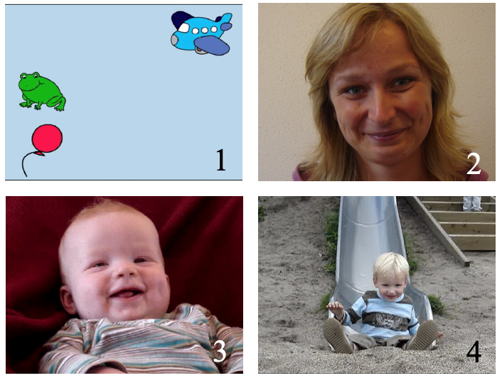
Figure 4.1: Visual stimuli presented during the pre- and posttest, habituation and test phase. Picture 1 is an example of the visual stimuli during pre-and posttest; 2 is an example of a female face used during habitation and test trials; 3 is a still of the attention getter between habituation trials and 4 is a still of the attention getter between test trials.
4.2.3 Procedure
Infants were seated on their caretaker’s lap in a sound-attenuated booth. As soon as infants looked towards the computer screen in front of them, the experimenter started the first trial. In each trial, the time the participant was looking at the screen was measured. Whenever the participant looked away for 2 consecutive seconds, the trial was ended; a new one started when the infant oriented to the screen again. There was no minimum looking time to the screen. Looking times were coded online using a button box connected to the computer controlling the experiment and acquiring data.
Pre- and posttest were used to gauge participants’ general attentiveness. If total looking time to the posttest stimulus was less than 50% of the total looking time to the pretest stimulus, the participant was considered to be showing a general loss of attention and was discarded for analysis. This was never the case in our sample (see Participants).
The habituation phase consisted of a maximum of 12 trials, with a maximum of 30 repetitions of a token per trial (ISI of 1 second) resulting in a total duration of approximately 48 seconds. A 65% habituation criterion was used to determine whether the participant had habituated. To determine whether the habituation criterion was met, a moving window was used (Figure 4.2). The mean looking times of the first three trials (1-3) was compared to the subsequent three trials (4-6): if looking time had decreased by (minimally) 35%, the criterion was met. If not, the mean looking time of trial 1-3 was compared to 5-7, 6-8, etc., and the same criterion applied, up until the final subset 10-12. Infants who did not meet the habituation criterion were not included in data analysis (\(n = 5\), see Participants). The selection of habituation stimuli (faap (/fa:p/) or feep (/fe:p/)) was counterbalanced between infants. Infants were presented with all four voices, in randomized order: in each block of four trials the infant heard all four voices but in randomized order within the blocks (see Figure 4.3).
The test phase included a fixed number of 12 trials, with a maximum number of 30 tokens per trial, resulting in a duration of approximately 48 seconds per trial. Houston et al. (2007) used 14 test trials (10 non-alternating and 4 alternating). We reduced the number of test phase trials and thus duration, because we know from experience that Dutch infants are not always able to sit through experiments that have the same duration as those conducted with infants in the US. Of these 12 test trials, four were alternating (e.g. /fe:p/-/fa:p/), and 8 non-alternating (e.g. /fa:p/-/fa:p/). The alternating and non-alternating trials were presented in a semi-fixed order: the first trial could be either alternating or non-alternating, which was counterbalanced. Three subsequent alternating trials occurred at positions: 5, 8 and 12. During the test phase a new token of one familiar speaker was introduced, either nonalternating or alternating (see Figure 4.3.
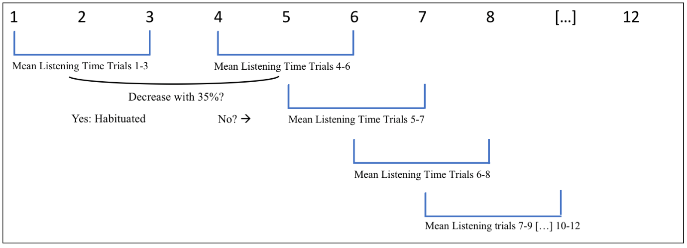
Figure 4.2: Visual depiction of the assessment of the (65%) habituation criterion
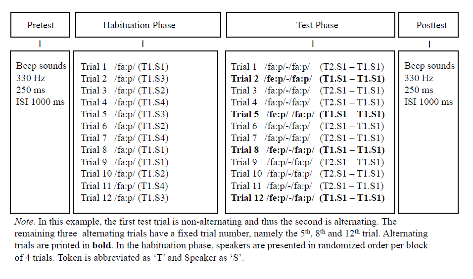
Figure 4.3: Schematic overview of the experimental procedure with reference to the auditory stimuli only. In this example, the first test trial is non-alternating and consequently the second is alternating. The remaining three alternating trials have a fixed number, viz. the 5th, the 8th and 12th trial. Alternating trials are printed in bold. Token is abbreviated as ‘T’ and Speakers as ‘S’
4.3 Results
4.3.1 Summary of the group data published in de Klerk et al. (2019)
The group-based data is presented in Figure 4.4 and Table 4.2. Mixed Modeling using SPSS (version 23) with Subjects as random factor, Trial Number as a repeated effect (covariance structure AR1), and Trial type (alternating vs. non-alternating) and Age as the fixed factors showed that at group level, infants between 6-10 months of age discriminated /fa:p/ from /fe:p/, at group level (de Klerk et al., 2019). In the current study we focus on the individual data.
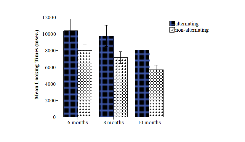
Figure 4.4: Raw mean looking times (milliseconds) to alternating and non-alternating trials per age group. Error bars represent Confidence Intervals (95%).
| Age Group | Infants | Alternating trials | Non-alternating Trials | Statistics | ||
|---|---|---|---|---|---|---|
| \(N\) | M (SD) | M (SD) | F | p | Cohen’s d | |
| 6 | 38 | 10.4 (8.6) | 7.9 (6.8) | 13.55 | < .001 | .31 |
| 8 | 44 | 9.7 (8.6) | 7.1 (6.7) | 21.74 | < .001 | .32 |
| 10 | 35 | 8.1 (5.6) | 5.7 (4.5) | 29.24 | < .001 | .45 |
| All | 117 | 9.4 (7.9) | 7.0 (6.3) | 62.70 | < .001 | .32 |
4.3.2 Data Screening
The raw looking times to alternating and non-alternating trials were not normally distributed; for this reason, a log transformation (Log10) was performed. After this transformation the skewness (.123, SE = .065) and kurtosis (.150, SE = .131) values were acceptable. We refer to the supplementary files for histograms of the raw and log transformed data (https://osf.io/ebrxy/).
4.3.3 Analysis 1: Linear Regression Model with Autoregressive (AR1) Error Structure
To assess individual performance, we used the same regression model with autoregressive effect as Houston et al. (2007),
\[\begin{equation} \begin{array}{l} y_t = b_0 + b_1 C_t + a_t \\ a_t = \begin{cases} \phi_1 a_{t-1} + e_t,& \text{if } t\geq 1\\ 0, & \text{otherwise} \end{cases} \end{array} \end{equation}\]
where subscript \(t\) denotes the trial number \(t=1,...,T\), \(y\), denotes the looking time of the trial, \(C\) denotes the condition (alternating or non-alternating) of the trial, \(e\) denotes the error term, \(\phi_1\) denotes the autoregressive factor. In this model \(b_1C_t\) accounts for the influence of the condition and \(b_1\) is interpreted as the difference in looking time for the two conditions. the dependence on the looking time of the previous trial is found in the specification of the error structure \(\phi_1a_{t-1}\). The error in the current time point (\(a_t\)) is dependent on the error of the previous time point (\(a_{t-1}\)), except for \(a_1\), because \(a_1\) is the first trial. There is no carry-over effect from the previous trial and no autoregressive effect. Looking times and statistical outcomes per infant are reported in Appendix A. Individual analyses show that condition effects were significant for 14 participants, implying that only 12% of the infants were able to discriminate between alternating and non-alternating trials. When we correct for multiple testing using the Benjamini-Hochberg procedure (Benjamini & Hochberg, 1995), this number decreases to 3 infants (3/117), a mere 3%.
Our results do not align with the results of the study of Houston et al. (2007), in which 80% (8/10) of the 9-month-old infants successfully discriminated the contrast. Applying the Benjamini-Hochberg correction for multiple testing to Houston et al. (2007) data did not make a difference in their outcomes, because of the few participants tested and the large effect of condition on looking times. Nevertheless, an analysis without having to correct for multiple testing is desirable and Bayesian modeling could be a solution.
4.3.4 Analysis 2: Hierarchical Bayesian Analysis
The analyses used in the paper by Houston et al. (2007) rely on separate regression analyses for each individual child. However, if we assume that infants are exchangeable within the same age group, that is, that they come from the same population, an alternative and more powerful approach is to model their looking times in a hierarchical (multilevel) structure. By modeling both the individual and group effects in one analysis instead of doing so for 117 separate analyses, one for each individual, part of the observed variance could be explained at the group level instead of trying to explain all variance at the individual level. As a result, we will have reduced uncertainty in our estimates for the individual parameters (Gelman, 2006a). Moreover, by using a Bayesian hierarchical analysis, we are able to obtain estimates for each of the individual and group parameters in one model without the need to correct for multiple testing (Gelman et al., 2012).
In our Bayesian hierarchical regression, we modelled the individual infant data in three groups based on their age (6, 8 and 10 months). We used the same model as before, namely a regression model with an AR1 error structure, with Log10 transformed looking times as outcomes and condition (alternating or non-alternating trial) as predictor. For all groups we obtained both group and individual estimates for the intercept (looking time alternating trials), the condition (difference in looking time between alternating and non-alternating trials) and the AR1 effect. Details on the priors, estimation, model fit and sensitivity analyses are given in the supplementary files on the Open Science Framework webpage for this study at (https://osf.io/ebrxy/) or in Appendix B. In short, we achieve a good model fit.
The parameter of interest was the condition parameter. This parameter allowed us to establish whether the looking times differed between the alternating and non-alternating condition for the individual infants. To keep the decision criterion as similar as possible to the previously described analyses, we checked how many of the infants included the value 0 in their 95% credibility interval (CI) for the condition parameter. For the 95% CI (the 0.025 and 0.975 quantiles of the posterior sample) we regard this interval as having a 95% probability of containing the unknown parameter value. In contrast, the 95% Confidence Interval in frequentist statistics relates to (potential) replications of the experiment and expresses the expectation that the interval contains the true parameter estimate in 95% of the experiments. In our study, the percentages of infants whose 95% CI did not include 0 are displayed per age group in Table 4.3. For the 10-months-olds we found that 77% discriminated between the alternating and non-alternating condition, and 53% of the 6-month-olds did, whilst for the 8-month-old infants this was only 27%.
| Frequentist (non-hierarchical) modeling | Bayesian Hierarchical modeling | |||
|---|---|---|---|---|
| Age Group | Participants | Uncorrected Successful Discrimination (%) | Corrected Successful Discrimination (%) | Infants without 0 in their 95% CI (%) |
| 6 | 38 | 2 (5) | 0 (0) | 20 (53) |
| 8 | 44 | 4 (9) | 2 (5) | 12 (27) |
| 10 | 35 | 8 (23) | 1 (3) | 27 (77) |
| Ttoal | 117 | 14 (12) | 3 (3) | 59 (50) |
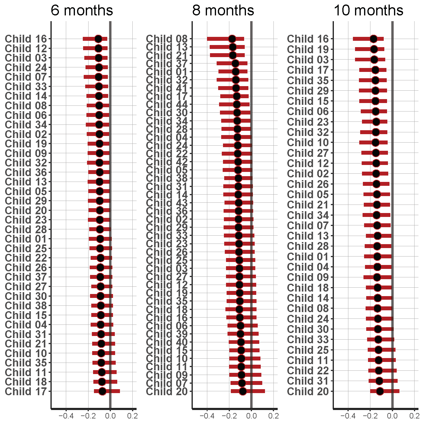
Figure 4.5: Results of the hierarchical model for each individual per age group. The black dots represent the median; the red bars represent the 95% Credibility Intervals.
Figure 4.5 shows the results of the hierarchical model for each individual per age group. Credibility Intervals for the 8-month-old infants show larger uncertainty for the estimates than for the other two age groups, especially the 6-month-olds. The group-estimated effect of condition, depicted in the left panel of Figure 4.6, increases with age. The estimated random effect for condition is largest in the 8-month-old group, which can be seen from the variance estimates in the right panel of Figure 4.6. Because the infants of the 8-month-old group differ more from one another than the infants in the other age groups, less shrinkage of estimates occurs and we remain more uncertain about their estimated condition effects. This outcome is visible in the larger credibility intervals for the infants in age group 8 compared to the other two age groups.
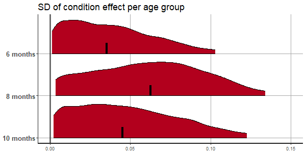
Figure 4.6: Group estimates for condition effects and variation per age group. The left panel shows the group estimates for condition effects. The right panel shows the standard deviation of the condition effect per age group. The densities, presented in red, represent the 95% credibility interval.
As part of the model assessment we conducted posterior predictive checks. These checks provide insight into the plausibility to the hypothesized and estimated model by drawing simulations from the posterior model. Figure 4.7 shows how well the model fits the data of a particular child, in this case child 16 in age group 6. Simulations are based on the posterior parameter estimates for this specific child at each specific measurement, taking into account the child-specific estimated looking times for (non-)alternating trials, the child-specific condition effect and the child-specific autoregressive effect. The posterior predictive \(p\)-value (ppp) indicates the proportion of simulated values for this measurement that are smaller than the observed value. If ‘ppp’ falls between 0.025 and 0.975 we conclude that our model provides an accurate prediction for this specific observation. Note that this specific child 16 is classified as non-discriminator and that all measurements are accurately captured by the model as shown by the blue bars in each histogram (Figure 4.7). For an example of a child classified as non-discriminator with less accurate model descriptions for the observed measurement see for instance child 17 from age group 10, measurements (trials) 5 and 7 (see https://osf.io/ebrxy/).
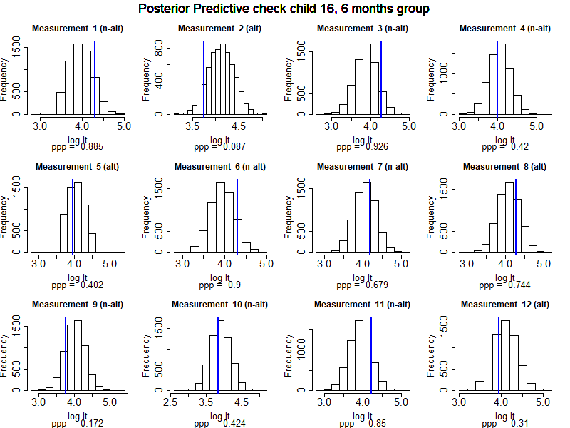
Figure 4.7: Posterior predictive simulations for child 16 in age group 6 for all 12 observed trials. Each histogram contains 6000 simulated values for that particular observation of that specific child based on the posterior parameter estimates. The blue vertical line denotes the actually observed value for the specific measurement.
To evaluate the effects of the hierarchical regression compared to modelling the individual regressions, we also ran Bayesian regression analyses with AR1 error structure without the multilevel structure. Figure 4.8 shows the estimates with their uncertainty for the condition parameter for all infants in age group 6 (only); the other groups show similar patterns. The figure shows that including the hierarchical structure reduced the uncertainty of the estimates markedly.
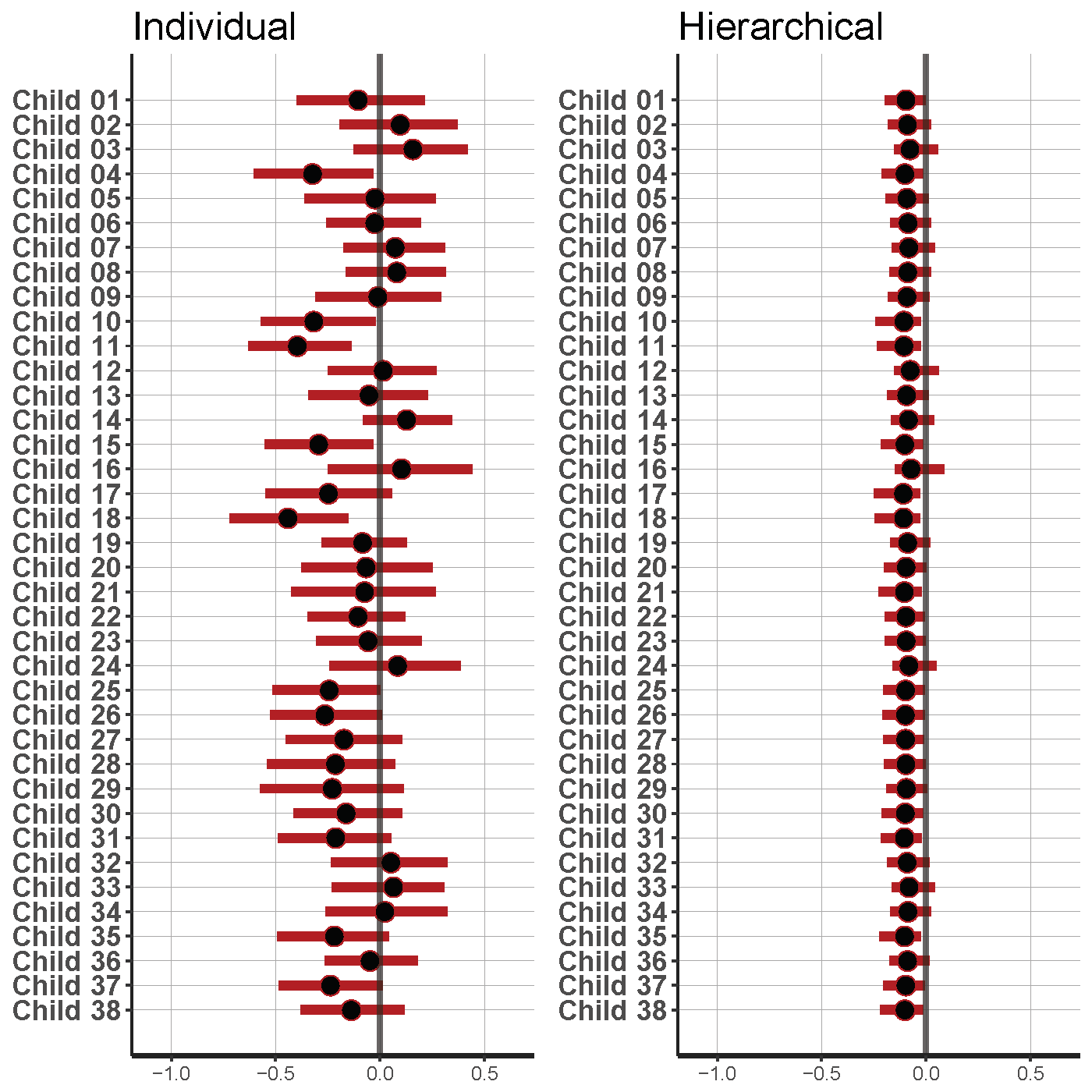
Figure 4.8: Comparison of results of individual and hierarchical analyses for condition parameter of each infant in the 6-month-olds group. The Hierarchical model reduces the uncertainty (95% CI represented by red bar) (median represented by the black dot) for the parameter estimates.
Table 4.4 displays the mean log-transformed looking time differences between the alternating and non-alternating trials for all individuals that did not include the value 0 in their 95% CI for the condition effect in the hierarchical regression. These raw data show the direction of the average difference in looking time between alternating and non-alternating trials, as well as the magnitude of the average difference between trial types. As can be seen, both looking time difference directions are present, meaning that the data set includes infants with on average longer looks to alternating trials as well as infants with on average longer looks to non-alternating trials. In addition, Table 4.4 shows that the magnitude of looking time differences between alternating and non-alternating trials shows considerable variation.
| Subject | Group | Difference | Subject | Group | Difference |
|---|---|---|---|---|---|
| Age | alternating - nonalternating | Age | alternating - nonalternating | ||
| child 02 | 6 | -.10 | child 41 | 8 | -.27 |
| child 03 | 6 | -.14 | child 44 | 8 | -.07 |
| child 05 | 6 | -.03 | child 01 | 10 | .12 |
| child 06 | 6 | .03 | child 02 | 10 | .13 |
| child 07 | 6 | -.10 | child 03 | 10 | -.09 |
| child 08 | 6 | -.01 | child 04 | 10 | .25 |
| child 09 | 6 | -.02 | child 05 | 10 | .11 |
| child 12 | 6 | -.05 | child 06 | 10 | .09 |
| child 13 | 6 | .02 | child 07 | 10 | .15 |
| child 14 | 6 | -.16 | child 08 | 10 | .26 |
| child 16 | 6 | -.13 | child 09 | 10 | .16 |
| child 19 | 6 | -.03 | child 10 | 10 | .11 |
| child 20 | 6 | .19 | child 12 | 10 | .20 |
| child 23 | 6 | .03 | child 13 | 10 | -.02 |
| child 24 | 6 | .09 | child 14 | 10 | .15 |
| child 29 | 6 | .11 | child 15 | 10 | -.12 |
| child 32 | 6 | .06 | child 16 | 10 | -.15 |
| child 33 | 6 | -.07 | child 17 | 10 | -.04 |
| child 34 | 6 | -.04 | child 18 | 10 | .14 |
| child 36 | 6 | .08 | child 19 | 10 | -.23 |
| child 01 | 8 | -.24 | child 21 | 10 | .03 |
| child 08 | 8 | -.36 | child 23 | 10 | .14 |
| child 13 | 8 | -.15 | child 26 | 10 | -.02 |
| child 17 | 8 | .19 | child 27 | 10 | .12 |
| child 20 | 8 | .48 | child 28 | 10 | .22 |
| child 21 | 8 | .04 | child 29 | 10 | -.10 |
| child 30 | 8 | -.10 | child 32 | 10 | .16 |
| child 32 | 8 | -.12 | child 34 | 10 | .36 |
| child 34 | 8 | -.11 | child 35 | 10 | .02 |
| child 37 | 8 | -.08 |
4.4 Discussion
The primary aim of this study was to determine if speech discrimination performance can be reliably assessed for individual infants in a habituation design. This is crucial for understanding individual developmental trajectories and in addressing potential clinical questions. In order to do so we used the experimental design, hybrid visual fixation (HVF), and statistical approach, linear regression modeling with autoregressive error structure, reported in Houston et al. (2007). Houston et al. (2007) found that 80% (8/10) of their 9-month-old participants discriminated the boodup - seepug contrast. Our study assessed individual native phoneme (/fa:p - /fe:p/) discrimination in Dutch infants aged 6, 8 and 10 months, using a slightly altered version of the HVF paradigm. When conducting the regression analysis that Houston et al. (2007) applied, we found that only 12% (14/117) of the infants discriminated the contrast. We were thus not able to replicate Houston et al. (2007)’s findings, using the same model as they did.
Houston et al. (2007) did not correct for multiple testing, but when such a correction is applied (as we did), it did not make a difference for the findings of the Houston et al. (2007) sample. For our study, however, the correction led to a reduction of the percentage of infants in whom discrimination could be attested to 3% (from 12%). Bayesian Hierarchical modeling provides both group and individual estimates using the same model and therefore has the advantage that it does not require correction for multiple testing. Using a hierarchical model with both the autoregressive effect (looking time decreases during test) and the inclusion of group information led to reduced uncertainty of the estimates of the condition effects (alternating versus non-alternating) at both the group and the individual level. The analysis returned a higher percentage (50%) of infants that showed evidence of discrimination. Evidence of discrimination is defined as the 95% credibility interval that does not include value 0 for the condition effect. For the 10-months-olds we found that 77% discriminated between faap and feep, while 53% of the 6-month-olds and only 27% of the 8-month-olds did. These individual discrimination outcomes are still lower than expected. We expected that most infants would show evidence of discrimination, regardless of age and we predicted discrimination percentages comparable to those obtained by Houston et al. (2007). Seventy-seven percent of the 10-months-old infants discriminated the contrast. This is comparable to findings of 9-month-olds in the study of Houston et al. (2007). It is conceivable that the design (14 alternating and non-alternating test trials) is more suitable for the older than for the younger infants.
Two design differences between the study by Houston et al. (2007) and ours could also account for the diverging results. First, Houston et al. (2007) used a word contrast, boodup - seepug, which differs markedly from the phonemic contrast /fa:p - fe:p/ we used. The more conspicuous word contrast may have elicited a larger difference between alternating and nonalternating trials. Second, Houston et al. (2007) used 14 test trials, two more non-alternating trials than we did. This might have caused a lower mean looking time to non-alternating trials, as infants’ internal representation of the old (non-alternating) stimulus might become stronger during test, which is expected to result in a larger increase in looking time to new stimuli (Sokolov, 1963). Still, infants of all age groups showed evidence of discrimination (de Klerk et al., 2019, and Figure 4.6 of this paper) and this does not seem to align with the lower percentage of infants significantly discriminating the contrast we observed in the current study. However, age-related enhancement of discrimination is shown by an increasing percentage of infants discriminating the contrast, which fits the theory of perceptual attunement (Maurer & Werker, 2014; Tsuji & Cristia, 2014).
Our individual analyses are an exploratory extension of the individual analyses done by Houston et al. (2007); we used Bayesian hierarchical modelling to assess if an infant can discriminate the two stimuli. The theoretical advantages of our approach have been discussed throughout the paper. The approach by Houston et al. (2007) and our approach lead to different conclusions for many infants in our study. Strictly speaking, our decision rule, i.e., discrimination is attested if the 95% CI does not include 0, is not an entirely proper method for hypothesis testing. Some shortcomings of forcing decision rules on parameter estimates are discussed in Lee (2018), where Bayes Factors are advocated. However, the application of Bayes Factors in the current setting would present serious challenges and there are arguments against them in general (Gelman et al., 2013). On the other hand, our approach is not unprecedented; Kruschke (2013), for example, used a similar approach as an alternative to t-tests, and Gelman & Tuerlinckx (2000) show that this approach reduces the chance of Type S (sign) errors in comparison to the classical framework. The decision rule we used could be used to infer discrimination.
The Bayesian hierarchical model presents a more reliable statistical approach: If measurements contain (substantial) noise, this negatively affects the reliability of a measurement. That is, if we measure the same construct multiple times we obtain different results. If we are able to reduce the noise, our measurement becomes less variable and will measure the same construct in a more stable manner over multiple times. By including hierarchical structures in our model we can capture part of the noise in our estimated looking times (see Figure 4.8). The reduction of the noise leads to less variable representations of the measurements which can be seen as an improvement of the reliability of the measurements (Gelman et al., 2012).
The current study aimed at assessing individual outcomes because looking time data is noisy and often challenging to interpret (Aslin & Fiser, 2005; Oakes, 2010). Nevertheless, studies do attempt to interpret these individual variations by, for instance, examining followup data and in retrospect analyze the infant looking time data (e.g. Newman et al., 2006), which at group level give some insight in the relations between early perception skills and later language development (Cristia et al., 2014). However, raw looking time data cannot be used to infer success or failure. In order to classify individuals as discriminators, data should be modelled and advanced statistical methods need to be applied. The method presented in this study allows us to classify individual infants as discriminators or non-discriminators. Moreover, the procedure allows us to investigate how well our model performs for each trial for each individual child using posterior predictive checks, an example can be seen in Figure 4.7. However, more research needs to be done to investigate replicability of the current study. Factors that will influence outcomes are, for example, sample size, as estimates will be more accurate with increased sample size, and the total number of data points per subject. Future research should also focus on the question whether classification as presented in this study is indeed of clinical value: do infants classified as discriminators have better language performance measured at a later age?
Taken together, assessing individual discrimination performance with an autoregressive model per individual without correcting for multiple testing is not an approach to be favored. On the other hand, if multiple testing is corrected for, significant results rely on sample size, because with each infant that is added another test should be run. Sample size influences the corrected alpha-level, which is arbitrary. A model in which all these issues can be tackled is the Bayesian Hierarchical model: we can account for a decrease in looking time (autoregressive effect); it includes group information in the hierarchical model; it does not require correction for multiple testing, and it provides more confidence in classifying infants as being able to discriminate a stimulus contrast or not. Our findings thus provide a step forward in assessing infants’ speech discrimination.
Ethics Statement
Informed consent was obtained from the caregiver before testing and the caregiver was allowed to retract this consent and participation any time during testing. The authors declare that the research was conducted in accordance with APA ethical standards as well as The Netherlands Code of Conduct for Scientific Practice issued in 2004 (revised in 2018 by the Association of Universities in the Netherlands (VSNU)).
Acknowledgments
We are grateful to the infants and their caregivers for participating. We would like to thank the student assistants Sule Kurtçebe, Tinka Versteegh, Lorijn Zaadnoordijk and Joleen Zuidema, who helped collecting data. We would like to thank Derek Houston for sharing some of his raw data with us (see Appendix A). This research was funded by The Netherlands Organization for Scientific Research (NWO). Grants nr. 360-70-270, awarded to. F.N.K. Wijnen and nr. VIDI-452-14-006, awarded to R. van de Schoot.
Appendix A
| Participant | Age | Condition | Difference | Statistics | |
|---|---|---|---|---|---|
| (months) | Alternating | Non-Alternating | Alt minus Non-alt | p_adj | |
| Child 10 | 6 | 4.05 | 3.74 | 0.31 | .012 |
| Child 38 | 6 | 3.71 | 3.59 | 0.12 | .022 |
| Child 31 | 6 | 3.92 | 3.69 | 0.22 | .055 |
| Child 4 | 6 | 4.26 | 3.98 | 0.28 | .055 |
| Child 18 | 6 | 4.43 | 4.08 | 0.35 | .062 |
| Child 35 | 6 | 3.95 | 3.67 | 0.29 | .074 |
| Child 15 | 6 | 4.22 | 3.98 | 0.24 | .100 |
| Child 25 | 6 | 4.26 | 3.94 | 0.32 | .113 |
| Child 29 | 6 | 4.06 | 3.95 | 0.11 | .128 |
| Child 37 | 6 | 4.24 | 4.02 | 0.22 | .133 |
| Child 17 | 6 | 3.74 | 3.58 | 0.16 | .134 |
| Child 11 | 6 | 4.34 | 3.99 | 0.35 | .14 |
| Child 26 | 6 | 4.2 | 4.06 | 0.14 | .211 |
| Child 30 | 6 | 3.88 | 3.75 | 0.13 | .23 |
| Child 14 | 6 | 3.61 | 3.76 | -0.16 | .258 |
| Child 3 | 6 | 3.8 | 3.94 | -0.14 | .278 |
| Child 28 | 6 | 4.16 | 3.9 | 0.26 | .293 |
| Child 22 | 6 | 3.9 | 3.8 | 0.1 | .295 |
| Child 7 | 6 | 3.82 | 3.91 | -0.1 | .335 |
| Child 2 | 6 | 3.57 | 3.67 | -0.1 | .347 |
| Child 33 | 6 | 3.87 | 3.94 | -0.07 | .406 |
| Child 19 | 6 | 4.01 | 4.04 | -0.03 | .416 |
| Child 27 | 6 | 4.05 | 3.99 | 0.06 | .46 |
| Child 8 | 6 | 3.77 | 3.78 | -0.01 | .524 |
| Child 16 | 6 | 4.02 | 4.15 | -0.13 | .56 |
| Child 1 | 6 | 3.97 | 3.87 | 0.1 | .603 |
| Child 13 | 6 | 3.84 | 3.82 | 0.02 | .665 |
| Child 20 | 6 | 3.96 | 3.78 | 0.19 | .675 |
| Child 21 | 6 | 3.55 | 3.47 | 0.07 | .675 |
| Child 32 | 6 | 3.72 | 3.66 | 0.06 | .723 |
| Child 23 | 6 | 3.79 | 3.76 | 0.03 | .725 |
| Child 6 | 6 | 4.09 | 4.05 | 0.03 | .748 |
| Child 24 | 6 | 4.21 | 4.12 | 0.09 | .773 |
| Child 36 | 6 | 3.99 | 3.91 | 0.08 | .847 |
| Child 5 | 6 | 3.7 | 3.73 | -0.03 | .85 |
| Child 12 | 6 | 4.19 | 4.23 | -0.05 | .857 |
| Child 9 | 6 | 3.79 | 3.82 | -0.02 | .899 |
| Child 34 | 6 | 3.88 | 3.92 | -0.04 | .905 |
| Child 9 | 8 | 4.42 | 3.7 | 0.72 | .001 |
| Child 7 | 8 | 3.76 | 3.3 | 0.46 | .001 |
| Child 20 | 8 | 3.97 | 3.49 | 0.48 | .022 |
| Child 15 | 8 | 3.94 | 3.55 | 0.38 | .031 |
| Child 38 | 8 | 3.43 | 3.51 | -0.08 | .051 |
| Child 19 | 8 | 3.95 | 3.74 | 0.21 | .053 |
| Child 10 | 8 | 4.01 | 3.73 | 0.28 | .057 |
| Child 27 | 8 | 4.2 | 4 | 0.2 | .062 |
| Child 35 | 8 | 4.36 | 3.96 | 0.4 | .067 |
| Child 17 | 8 | 4.3 | 4.11 | 0.19 | .092 |
| Child 40 | 8 | 4.15 | 3.78 | 0.37 | .098 |
| Child 29 | 8 | 4.24 | 4.02 | 0.22 | .142 |
| Child 5 | 8 | 4.13 | 4 | 0.13 | .144 |
| Child 11 | 8 | 3.82 | 3.47 | 0.35 | .153 |
| Child 25 | 8 | 3.88 | 3.72 | 0.16 | .160 |
| Child 6 | 8 | 3.72 | 3.54 | 0.18 | .160 |
| Child 12 | 8 | 3.85 | 3.7 | 0.15 | .202 |
| Child 13 | 8 | 3.82 | 3.97 | -0.15 | .242 |
| Child 41 | 8 | 3.68 | 3.95 | -0.27 | .254 |
| Child 8 | 8 | 3.68 | 4.04 | -0.36 | .294 |
| Child 16 | 8 | 4.25 | 4 | 0.25 | .319 |
| Child 36 | 8 | 4.06 | 3.94 | 0.12 | .332 |
| Child 3 | 8 | 3.92 | 3.8 | 0.12 | .354 |
| Child 18 | 8 | 3.9 | 3.69 | 0.21 | .387 |
| Child 23 | 8 | 4.04 | 3.85 | 0.19 | .397 |
| Child 26 | 8 | 3.84 | 3.69 | 0.15 | .420 |
| Child 39 | 8 | 3.79 | 3.59 | 0.2 | .440 |
| Child 31 | 8 | 4.18 | 4.03 | 0.15 | .483 |
| Child 4 | 8 | 4.12 | 3.98 | 0.13 | .499 |
| Child 1 | 8 | 3.8 | 4.04 | -0.24 | .592 |
| Child 33 | 8 | 3.88 | 3.71 | 0.17 | .612 |
| Child 21 | 8 | 4.23 | 4.19 | 0.04 | .672 |
| Child 2 | 8 | 3.7 | 3.7 | 0.01 | .692 |
| Child 14 | 8 | 3.53 | 3.6 | -0.07 | .712 |
| Child 22 | 8 | 3.87 | 3.87 | 0 | .716 |
| Child 32 | 8 | 3.89 | 4.01 | -0.12 | .728 |
| Child 44 | 8 | 3.81 | 3.88 | -0.07 | .745 |
| Child 30 | 8 | 3.7 | 3.8 | -0.1 | .768 |
| Child 43 | 8 | 3.48 | 3.54 | -0.05 | .786 |
| Child 28 | 8 | 3.81 | 3.78 | 0.03 | .904 |
| Child 37 | 8 | 4.13 | 4.22 | -0.08 | .909 |
| Child 34 | 8 | 3.55 | 3.66 | -0.11 | .925 |
| Child 42 | 8 | 3.74 | 3.75 | -0.01 | .937 |
| Child 24 | 8 | 4.12 | 3.87 | 0.25 | .947 |
| Child 20 | 10 | 4.14 | 3.52 | 0.62 | .001 |
| Child 34 | 10 | 4.23 | 3.88 | 0.36 | .003 |
| Child 22 | 10 | 4.15 | 3.66 | 0.49 | .005 |
| Child 24 | 10 | 3.96 | 3.67 | 0.29 | .014 |
| Child 30 | 10 | 3.85 | 3.53 | 0.32 | .016 |
| Child 32 | 10 | 4.01 | 3.85 | 0.16 | .018 |
| Child 31 | 10 | 4.04 | 3.54 | 0.5 | .020 |
| Child 8 | 10 | 4.03 | 3.76 | 0.26 | .043 |
| Child 9 | 10 | 3.7 | 3.54 | 0.16 | .076 |
| Child 25 | 10 | 3.98 | 3.66 | 0.32 | .096 |
| Child 14 | 10 | 3.67 | 3.52 | 0.15 | .129 |
| Child 28 | 10 | 3.97 | 3.75 | 0.22 | .155 |
| Child 11 | 10 | 3.57 | 3.45 | 0.12 | .195 |
| Child 10 | 10 | 3.93 | 3.82 | 0.11 | .197 |
| Child 12 | 10 | 4.04 | 3.83 | 0.2 | .219 |
| Child 19 | 10 | 3.57 | 3.81 | -0.23 | .262 |
| Child 2 | 10 | 3.99 | 3.86 | 0.13 | .266 |
| Child 4 | 10 | 4.03 | 3.79 | 0.25 | .29 |
| Child 7 | 10 | 3.97 | 3.82 | 0.15 | .306 |
| Child 16 | 10 | 3.81 | 3.97 | -0.15 | .327 |
| Child 5 | 10 | 3.93 | 3.81 | 0.11 | .344 |
| Child 3 | 10 | 3.84 | 3.93 | -0.09 | .395 |
| Child 18 | 10 | 3.51 | 3.37 | 0.14 | .420 |
| Child 35 | 10 | 4.15 | 4.13 | 0.02 | .520 |
| Child 15 | 10 | 3.6 | 3.72 | -0.12 | .592 |
| Child 27 | 10 | 3.65 | 3.52 | 0.12 | .599 |
| Child 29 | 10 | 3.67 | 3.77 | -0.1 | .601 |
| Child 21 | 10 | 3.87 | 3.84 | 0.03 | .641 |
| Child 23 | 10 | 3.99 | 3.85 | 0.14 | .734 |
| Child 1 | 10 | 3.83 | 3.71 | 0.12 | .832 |
| Child 17 | 10 | 3.9 | 3.93 | -0.03 | .891 |
| Child 6 | 10 | 3.9 | 3.81 | 0.09 | .899 |
| Child 33 | 10 | 3.73 | 3.61 | 0.12 | .902 |
| Child 13 | 10 | 3.44 | 3.46 | -0.02 | .955 |
| Child 26 | 10 | 3.59 | 3.61 | -0.02 | .996 |
| 768 | 9 (Houston) | 25800 | 8380 | 17420 | .000 |
| 929 | 9 (Houston) | 11614 | 7843 | 3771 | .056 |
| 668 | 9 (Houston) | 12425 | 13060 | -635 | .336 |
| 762 | 9 (Houston) | 8671 | 6743 | 1928 | .529 |
Appendix B
4.4.1 Software
We used R version 3.4.3 (R Core Team, 2017b) and rstan version 2.17.3 (Stan Development Team, 2018b) to estimate the models. We used shinystan version 2.4.0 (Gabry, 2018) to asses model convergence. The packages ggplot2 version 2.2.1 (Wickham et al., 2019) and gridExtra version 2.3 (Auguie, 2017) were used in creating our figures and the package foreign version 0.8-69 (R Core Team, 2017a) was used to load the data into R.
4.4.2 Priors
We specified half-cauchy priors with location of 0 and scale 2.5 on the variance parameters in accordance with recommendations by Gelman (2006b). All other parameters are modelled with uninformative priors given the scale of the data, namely normal priors with a mean of 0 and a standard deviation of 100.
4.4.3 Estimation and Convergence
We ran 4 chains using 1000 warmup samples and 2500 iterations each. We looked at several indicators to check if our model had converged and if the model was appropriate. The \(\hat{R}\) (< 1.01), Monte Carlo standard error (< 5%) and effective sample size (>10%) did not display problematic signs for any of the parameters. No divergent transitions were found and the energy diagnostic for the Hamiltonian Monte Carlo looked fine (Betancourt, 2017).
4.4.4 Posterior predictive check
To see if the model was appropriate for the data we performed posterior predictive checks for each observation for each child. That is, we simulated data using the estimated model and looked if the original data would be surprising given the model. If there were few discrepancies between the model generated data and the original data the model was assumed to be appropriate. An example of such posterior predictive checks can be seen in Figure 4.9. For a pdf including all posterior predictive checks see the document “Posterior_Predictives.pdf” in the data Archive on the Open Science Framework (OSF) webpage for this study at https://osf.io/ebrxy/. Only 3.3% of the observations did not pass this check and there did not seem to be a pattern in which observations did not pass the check. We therefore conclude that the model described the data well.
4.4.5 Sensitivity Analysis
Figure 4.10 shows the effects for the condition parameter estimates if we change the priors on the group SD parameters. We compare a uniform (0, Inf), a half Cauchy (0, 2.5) an inverse gamma (0.1, 0.1) and an inverse gamma (0.5, 0.5) prior. We see that the variation for the individuals stays about the same for the uniform and Cauchy prior but increases a bit if we use the inverse gamma (0.1, 0.1) and somewhat more if we use the inverse gamma (0.5, 0.5) prior. This is due to a prior data conflict for the inverse gamma priors and the data. The data are on the log10 scale and thus we obtain small values with small SD estimates. The estimates are so small that their values are extremely unlikely given the inverse gamma prior specifications. (smaller than 1% chance for inverse gamma (0.1, 0.1) and smaller than 0.001% for inverse gamma (0.5, 0.5)). These priors thus artificially increase variance between individuals as you see in the figure and are not uninformative for this data set. A visual representation of the priors and the lack of support of the inverse gamma priors on parameter space with very small values can be seen in Figures 4.11. The Cauchy and uniform prior are uninformative given the scale of the data but are not in disagreement with the data. They cause stable results over different choices thus encouraging us to trust the results from the analyses with the half Cauchy(0, 2.5) prior.
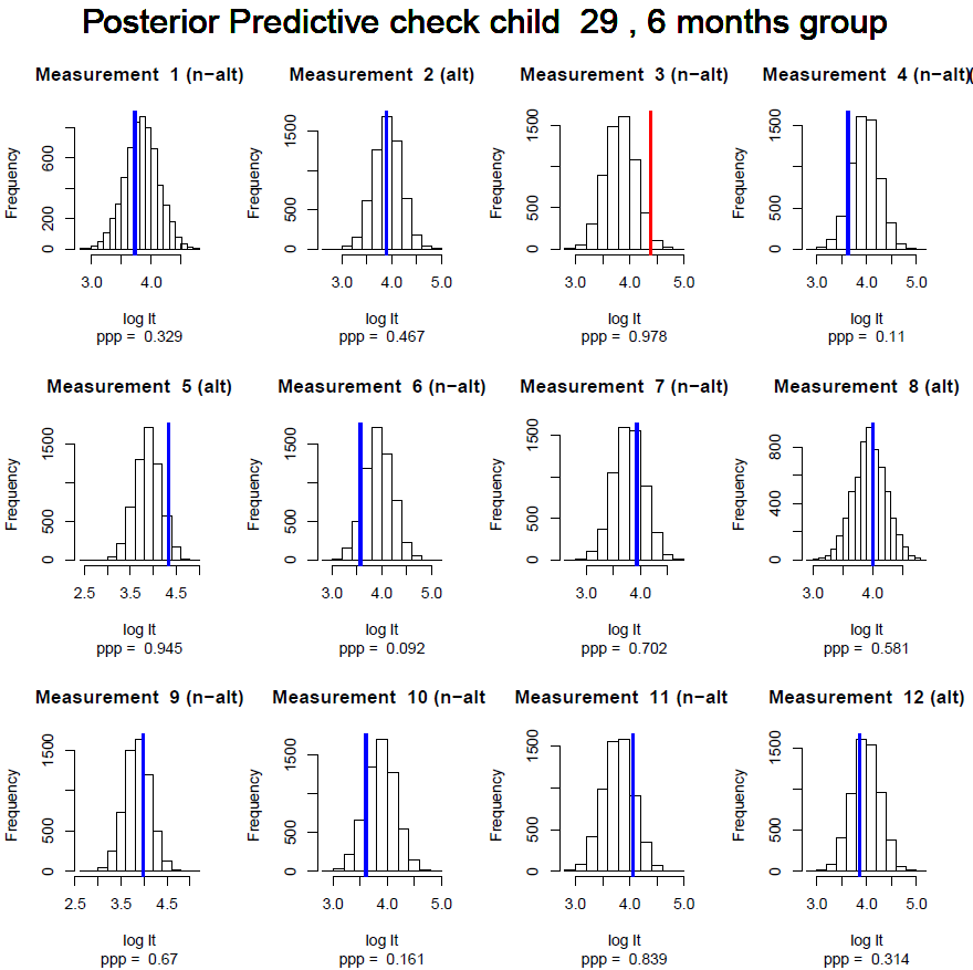
Figure 4.9: Example of posterior predictive check. 1500 Samples are generated based on the model estimates for each measurement for each individual. The original observation is marked with a blue line if it falls within the 95% interval of the observations and with red if it falls outside. If the model is a good model the observed data should not be surprising given the model. As such, if the model is good we should expect few observations that we cannot explain and thus few ‘red’ lines in the histograms.
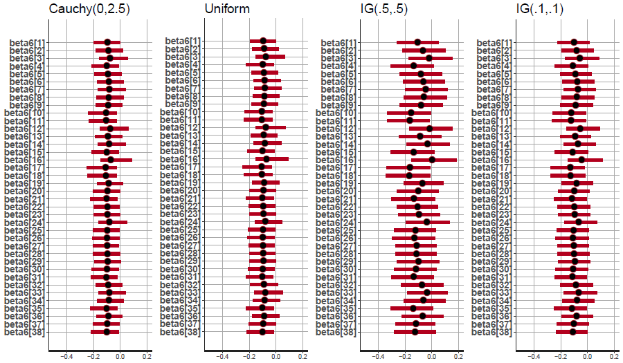
Figure 4.10: Results of the sensitivity analyses regarding the effects of the choice of the prior on the group standard deviation parameters on the condition parameter in which we a interested for this study.
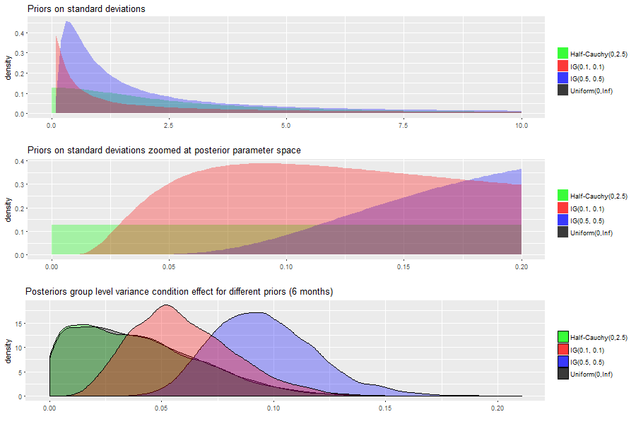
Figure 4.11: Visualization of the priors used in the sensitivity analysis, also zoomed at the posterior parameter space that is relevant and we also present the resulting posterior distributions if these priors are used.
References
Altvater-Mackensen, N., & Grossmann, T. (2015). Learning to match auditory and visual speech cues: Social influences on acquisition of phonological categories. Child Development, 86(2), 362–378.
Aslin, R. N., & Fiser, J. (2005). Methodological challenges for understanding cognitive development in infants. Trends in Cognitive Sciences, 9(3), 92–98.
Auguie, B. (2017). GridExtra: Miscellaneous functions for "grid" graphics. Retrieved from https://CRAN.R-project.org/package=gridExtra
Benjamini, Y., & Hochberg, Y. (1995). Controlling the false discovery rate: A practical and powerful approach to multiple testing. Journal of the Royal Statistical Society: Series B (Methodological), 57(1), 289–300.
Betancourt, M. (2017). A conceptual introduction to Hamiltonian Monte Carlo. arXiv Preprint arXiv:1701.02434.
Colombo, J., & Mitchell, D. W. (2009). Infant visual habituation. Neurobiology of Learning and Memory, 92(2), 225–234.
Cristia, A. (2011). Fine-grained variation in caregivers’/s/predicts their infants’/s/category. The Journal of the Acoustical Society of America, 129(5), 3271–3280.
Cristia, A., Seidl, A., Junge, C., Soderstrom, M., & Hagoort, P. (2014). Predicting individual variation in language from infant speech perception measures. Child Development, 85(4), 1330–1345.
Cristia, A., Seidl, A., Singh, L., & Houston, D. (2016). Test-retest reliability in infant speech perception tasks. Infancy, 21(5), 648–667.
de Klerk, M., de Bree, E., Kerkhoff, A., & Wijnen, F. (2019). Lost and Found: Decline and Reemergence of Non-Native Vowel Discrimination in the First Year of Life. Language Learning and Development, 15(1), 14–31.
Dijkstra, C., & Fikkert, J. (2011). Universal Constraints on the Discrimination of Place of Articulation? Asymmetries in the Discrimination of ’paan’and ’taan’ by 6-month-old Dutch Infants.
Gabry, J. (2018). Shinystan: Interactive Visual and Numerical Diagnostics and Posterior Analysis for Bayesian Models. Retrieved from https://CRAN.R-project.org/package=shinystan
Gelman, A. (2006a). Multilevel (hierarchical) modeling: What it can and cannot do. Technometrics, 48(3), 432–435.
Gelman, A. (2006b). Prior distributions for variance parameters in hierarchical models (comment on article by Browne and Draper). Bayesian Analysis, 1(3), 515–534.
Gelman, A., Carlin, J. B., Stern, H. S., Dunson, D. B., Vehtari, A., & Rubin, D. B. (2013). Bayesian data analysis. CRC press.
Gelman, A., Hill, J., & Yajima, M. (2012). Why we (usually) don’t have to worry about multiple comparisons. Journal of Research on Educational Effectiveness, 5(2), 189–211.
Gelman, A., & Tuerlinckx, F. (2000). Type S error rates for classical and Bayesian single and multiple comparison procedures. Computational Statistics, 15(3), 373–390.
Horn, D. L., Houston, D. M., & Miyamoto, R. T. (2007). Speech discrimination skills in deaf infants before and after cochlear implantation. Audiological Medicine, 5(4), 232–241.
Houston, D. M., Horn, D. L., Qi, R., Ting, J. Y., & Gao, S. (2007). Assessing speech discrimination in individual infants. Infancy, 12(2), 119–145.
Houston-Price, C., & Nakai, S. (2004). Distinguishing novelty and familiarity effects in infant preference procedures. Infant and Child Development: An International Journal of Research and Practice, 13(4), 341–348.
Junge, C., & Cutler, A. (2014). Early word recognition and later language skills. Brain Sciences, 4(4), 532–559.
Kruschke, J. K. (2013). Bayesian estimation supersedes the t test. Journal of Experimental Psychology: General, 142(2), 573.
Lee, M. D. (2018). Bayesian methods in cognitive modeling. Stevens’ Handbook of Experimental Psychology and Cognitive Neuroscience, 5, 1–48.
Liu, L., & Kager, R. (2015). Bilingual exposure influences infant VOT perception. Infant Behavior and Development, 38, 27–36.
Liu, L., & Kager, R. (2016). Perception of a native vowel contrast by Dutch monolingual and bilingual infants: A bilingual perceptual lead. International Journal of Bilingualism, 20(3), 335–345.
Maurer, D., & Werker, J. F. (2014). Perceptual narrowing during infancy: A comparison of language and faces. Developmental Psychobiology, 56(2), 154–178.
Melvin, S. A., Brito, N. H., Mack, L. J., Engelhardt, L. E., Fifer, W. P., Elliott, A. J., & Noble, K. G. (2017). Home environment, but not socioeconomic status, is linked to differences in early phonetic perception ability. Infancy, 22(1), 42–55.
Molfese, D. L. (2000). Predicting dyslexia at 8 years of age using neonatal brain responses. Brain and Language, 72(3), 238–245.
Newman, R., Ratner, N. B., Jusczyk, A. M., Jusczyk, P. W., & Dow, K. A. (2006). Infants’ early ability to segment the conversational speech signal predicts later language development: A retrospective analysis. Developmental Psychology, 42(4), 643.
Oakes, L. M. (2010). Using habituation of looking time to assess mental processes in infancy. Journal of Cognition and Development, 11(3), 255–268.
R Core Team. (2017a). Foreign: Read Data Stored by ’Minitab’, ’S’, ’SAS’, ’SPSS’, ’Stata’, ’Systat’, ’Weka’, ’dBase’, ... Retrieved from https://CRAN.R-project.org/package=foreign
R Core Team. (2017b). R: A Language and Environment for Statistical Computing. Vienna, Austria: R Foundation for Statistical Computing. Retrieved from https://www.R-project.org/
Sokolov, E. N. (1963). Perception and the conditioned reflex. New York, NY: Macmillan.
Stan Development Team. (2018b). RStan: The R interface to Stan. Retrieved from http://mc-stan.org/
Tsao, F., Liu, H., & Kuhl, P. K. (2004). Speech perception in infancy predicts language development in the second year of life: A longitudinal study. Child Development, 75(4), 1067–1084.
Tsuji, S., & Cristia, A. (2014). Perceptual attunement in vowels: A meta‐analysis. Developmental Psychobiology, 56(2), 179–191.
Wickham, H., Chang, W., Henry, L., Pedersen, T. L., Takahashi, K., Wilke, C., … Yutani, H. (2019). Ggplot2: Create elegant data visualisations using the grammar of graphics. Retrieved from https://CRAN.R-project.org/package=ggplot2