1 Introduction

1.1 Bayesian Statistics

We all have to make decisions whilst facing uncertainty and incomplete information. To help us interpret and organize available information we use statistics. One framework that is often used to plan the optimal course of action is Bayesian statistics.

Bayesian statistics offers a way to describe our state of knowledge in terms of probability (Jaynes, 1996). Moreover, it can be seen as an extension of logic (Jaynes, 2003). In addition, Bayesian statistics describes how we ought to learn (Lindley, 2013). We can do so by using probability distributions to describe our state of knowledge about a parameter. This can be done both before we observe new data, i.e. by means of a prior distribution of probability concerning the parameter, or after we have observed new data and we have updated our state of knowledge, i.e. the posterior distribution of probability concerning the parameter.

To make this more intuitive I very briefly describe learning via Bayesian statistics. I use the example describing how we could learn about the unknown proportion of a sequence of ‘Bernoulli trials’ that result in either 0 or 1, or in case of a coin, tails (\(T\)) for 0 or head (\(H\)) for 1. We say that \(\theta\) is the proportion of coin flips resulting in heads facing upwards. It turns out that we can use the Beta distribution in a very convenient way to update our beliefs, or state of knowledge, concerning \(\theta\). That is, we can express which values are consistent with both our prior state of knowledge and the newly observed data (Jaynes, 1996). The distribution of probability indicates which values are most consistent with both sources. For mathematical details see for instance Gelman et al. (2013 Chapter 2). The intuition is as follows: the Beta distribution has two parameters, \(\alpha\) and \(\beta\), which can be interpreted as follows in our example; there have ‘Bernoulli trials’, and \(\alpha - 1\) of them have been a success whilst \(\beta - 1\) of them have been a failure. In other words we have observed heads \(\alpha - 1\) times and tails \(\beta - 1\) times.

Now let us start with a prior state of ignorance, we have neither observed head nor tails before. We then specify a \(Beta(\alpha = 1, \beta = 1)\) prior distribution. It turns out that this neatly coincides with an initial state of ignorance. Every proportion in the interval from 0 up to 1 is assigned equal probability to be the value for \(\theta\) based on no initial evidence, see Figure 1.1 panel A. Now we observe heads four times and tails once (\(THHHH\)) in the first five trials and we learn from this data such that we update to a posterior distribution represented by a \(Beta(\alpha = 5, \beta = 2)\), which can be seen in Figure 1.1 panel B. Before we observe more trials and new data we have an updated state of belief. The posterior distribution can become our new prior distribution, which we, in turn, update with new information to obtain a new posterior distribution. This is what happens in panels C and D of Figure 1.1 where we in turn observe \(HTHHT\) and \(THTTH\) to come to a \(Beta(\alpha = 8, \beta = 4)\) as a posterior in panel C and a \(Beta(\alpha = 10, \beta = 7)\) as posterior in panel D. After 15 trials, and without initial prior knowledge, slightly more heads were observed than tails, thus values just above a proportion of .5 are assigned the largest probability. However, given the few trials that we observed, a wide range of possible values for the proportion of coin flips resulting in heads facing upwards are still assigned probability. Note too, that nowhere do I state which value for \(\theta\) I used to simulate these results, for in practice this is unknown and the best we can do is what we just did, use the knowledge available to us to assign probabilities to values for \(\theta\).

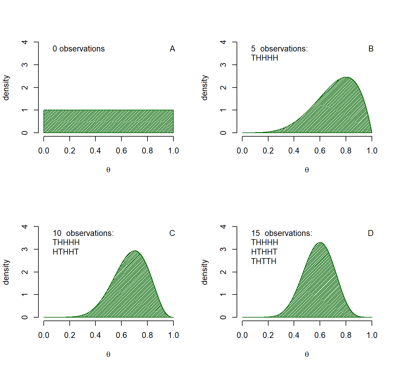
Figure 1.1: Example of Bayesian updating. Panel A shows a \(Beta(\alpha = 1, \beta = 1)\) distribution representing a prior state of knowledge equal to ignorance. Panels B, C and D show how the state of knowledge updated after new data is observed, each time the previous panel is the prior belief for the next panel, combined with the information from five new observations.

Now, let us suppose that we did not have an initial state of ignorance. The prior need not be ignorance as we noticed when the previous posterior became our new prior each time. Would of belief differ if we had more initial information? Figure 1.2 shows learning from the same data as in the example presented in Figure 1.1 with our initial state of knowledge expressed by a \(Beta(\alpha = 51, \beta = 51)\) distribution. In other words, before the new trials we had initial information equivalent to 100 previous coin flips that were distributed equally between head and tails. The new data is very much in line with our previous data and we only slightly adjust our beliefs, assigning even more probability to values near .5.

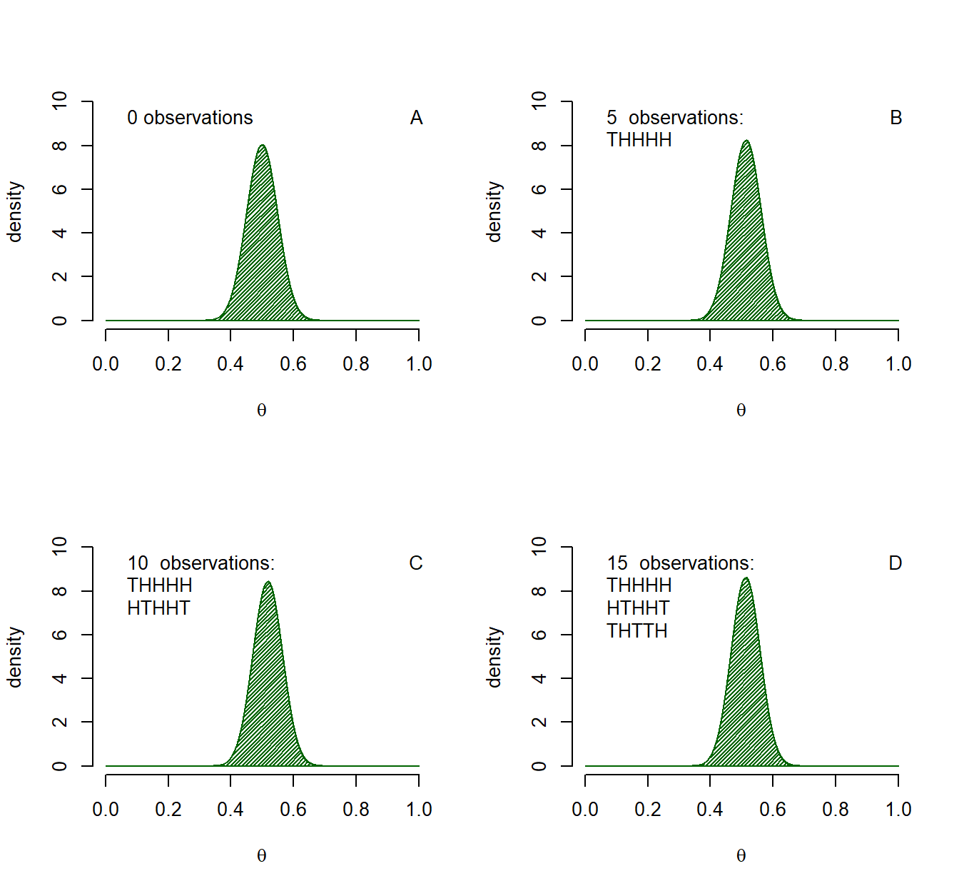
Figure 1.2: Example of Bayesian updating. Panel A shows a \(Beta(\alpha = 51, \beta = 51)\) distribution. This is updated using the same data as in Figure 1.1, only the initial prior contains more information.

All of this wonderful nuanced theory is historically summarized by a single equation. The reason for showing you this formula only after the examples, is not to get distracted by the mathematics for those readers not working with statistics every day. For those who do use statistics often, there are many books written in much more detail on this subject that yield a more complete overview (e.g. Gelman et al., 2013; Jaynes, 2003; Kaplan, 2014; Lindley, 2013; Lynch, 2007; Ntzoufras, 2011; Press, 2009). Without further ado, Bayes’ Theorem

\[\begin{equation} p(A|BC) = P(A|C)\frac{P(B|AC)}{P(B|C)} \tag{1.1} \end{equation}\]

where \(A\), \(B\) and \(C\) are different propositions, \(p(A|C)\) describes the prior distribution of probability concerning \(A\), given that we know \(C\). \(p(A|BC)\) is the posterior distribution of probability concerning \(A\), updated with the new information that is provided to us by \(B\). Note that \(C\) here has the interpretation of what we know about \(A\) before learning about, or obtaining, the information from \(B\). In the previous example, \(\theta\) took on the role of \(A\) and the new trials took on the role of \(B\). \(C\), in the first example, expressed that we knew that \(\theta\) was a proportion which can only take on values in the interval from 0 up to 1. Equation (1.1) describes how we can learn about \(A\), how we ought to update our beliefs in the light of new data. It also makes it explicit that this learning effect is dependent on our prior knowledge, just like in the example of Figures 1.1 and 1.2 Again, the aim here is not to expand on the mathematics, but merely to provide some initial intuition about the concept of learning using Bayes’ rule. Next, we turn to the implementation of the concept of prior knowledge, how can we formalize our prior distribution of probability concerning \(A\) given that we know \(C\).

1.2 Prior Information

The topic of prior information in Bayesian statistics is a field of study all on it’s own. To illustrate this, note that Tuyl, Gerlach, & Mengersen (2008) wrote a full paper, discussing only the choice of prior for extreme cases of our example above. There are heavy discussions and different schools of thought, roughly divided into “objective” (e.g. Berger, 2006) and “subjective” (e.g. de Finetti, 1974; Goldstein, 2006) camps. Discussing the differences within, let alone between, these different approaches is way to much to get into at this point. Simply listing names of different approaches to objective Bayesian priors takes up an extensive paragraph (Berger, 2006, pp. 387–388) and for a discussion about the (dis)advantages of both method I refer the reader to Chapter 5 of Press (2009). For the reader it suffices to know that in this dissertation we certainly specify priors that would be considered more in line with the “subjective” school of Bayesian analysis, even if we do not always use these priors to be updated with new data.

Now let us briefly consider three types of information that could be included in a prior distribution of probability. First, previous research can inform us about certain parameters and including this information in future analyses seems in line with our idea of leaning. In Section 5.4 of Spiegelhalter, Abrams, & Myles (2004) they provide a very nice overview on how to include results of previous studies based on similarity, exchangability and bias considerations. It is described not only how you could include information from previous studies if they are exactly on the same topic, but also how to do so if the research differs in specific ways. Second, logical considerations can be taken into account, e.g. in the coin flipping example we know that a proportion lies between 0 and 1 and no values outside the interval between those two will be assigned any probability. In a similar fashion we could incorporate information with respect to our measurements, e.g. no negative values for temperature measured in Kelvin, or when calculating air pollution in a city that we do live in, the amount of matter in the air cannot be so much that we could not breath and live there. Third, information gathered from an expert, or as put by the Cambridge English Dictionary (2019); “a person with a high level of knowledge or skill relating to a particular subject or activity”. This particular knowledge can be translated, or elicited, to be expressed in the form of distribution of probability. There are surely more sources of information to inform our prior probability distributions besides previous research, logical considerations and expert knowledge, but as this dissertations involves experts quite a bit I will elaborate on that specific case somewhat more.

1.3 Expert Elicitation

The process of creating a probabilistic representation of an experts’ beliefs is called elicitation (O’Hagan et al., 2006). There is an extensive history of expert elicitation across many different disciplines of sciences (Cooke & Goossens, 2008; Gosling, 2018; O’Hagan et al., 2006, Chapter 10). Expert judgements are for instance used in the case that there is no actual data available (Hald et al., 2016) or to add information to small sample data (Kadane, 1994). However, with many examples, covering many disciplines, expert knowledge still does not seem to be used in the social sciences with van de Schoot, Winter, Ryan, Zondervan-Zwijnenburg, & Depaoli (2017) finding only two use cases in the past 25 years of Bayesian statistics in Psychology.

One of the reasons for this limited use can perhaps be found in the traditional way of eliciting expert judgements. One of the traditional ways is to elicit three quantiles from an experts concerning the distribution of probability over a specific parameters (O’Hagan et al., 2006, Chapter 5). These quantiles are then used to determine the distribution that fits best with these described value, and that distribution is used to represent an experts’ beliefs. The questions to the experts would be for instance the following:

"Q1: Can you determine a value (your median) such that X is equally likely to be less than or greater than this point?

Q2: Suppose you were told that X is below your assessed median. Can you now determine a new value (the lower quartile) such that it is equally likely that X is less than or greater than this value?

Q3: Suppose you were told that X is above your assessed median. Can you now determine a new value (the lower quartile) such that it is equally likely that X is less than or greater than this value?"

O’Hagan et al. (2006), p. 101

We believe that this rather abstract thinking in terms of quantiles of distributions might be hard for some experts, depending on their experience with statistics and mathematical background. This naturally bring us to the following section and the outline of this dissertation, how is it that we propose to use expert elicitation in the social sciences and what do we propose to do with this source of additional information.

1.4 Aims and Outline

In this dissertation it is discussed how one can capture and utilize alternative sources of (prior) information compared to traditional method in the social sciences such as survey research. Specific attention is paid to expert knowledge.

In Chapter 2 we propose an elicitation methodology for a single parameter that does not rely on specifying quantiles of a distribution. The proposed method is evaluated using a user feasibility study, a partial validation study and an empirical example of the full elicitation method.

In Chapter 3 it is investigated how experts’ knowledge, as alternative source of information, can be contrasted with traditional data collection methods. At the same time, we explore how experts can be assessed and ranked borrowing techniques from information theory. We use the information theoretical concept of relative entropy or Kullback-Leibler divergence which assesses a loss of information when approximating one distribution by another. For those familiar with the concept of model selection, Akaike’s Information Criterion is an approximation of this (Burnham & Anderson, 2002, Chapter 2).

In Chapter 4 an alternative way of enhancing the amount of information in a model is proposed. We introduce Bayesian hierarchical modelling to the field of infants’ speech discrimination analysis. This technique is not new on it’s own but was not applied to this field. Implementing this type of modelling enables individual analyses within a group structure. By taking the hierarchical structure of the data into account we can make the most of the, on individual level, small noisy data sets. The analysis methodology estimates if individuals are (dis)similar and takes this into account for all individuals in one single model. Essentially, the estimated group effects serve as priors for the individual estimates. Moreover, we do not need to do a single hypothesis test for every child, which was the most advanced individual analysis in the field up to now, going back to 2007 (Houston, Horn, Qi, Ting, & Gao, 2007).

In Chapter 5 we reflect on issues that come along with the estimation of increasingly complicated models. Techniques and software for estimating more complex models, such as proposed in Chapter 4, need to be carefully used and the results of the analyses need to be carefully checked. But what to do when things actually go awry in your analysis? We show how even with weakly informative priors, adding the information that is available to us, sometimes we do not get a solution with our analysis plan. We guide the reader on what to do when this occurs and where to look for clues and possible causes. We provide some guidance and a textbook example that for once shows things not working out the way you would like. We believe this is important as there are few examples of this.

In Chapter 6 we combine the previous chapters. We take more complex models and get experts to specify beliefs with respect to these models. We extend the method developed in Chapter 2 to elicit experts’ beliefs with respect to a hierarchical model, which is used in Chapters 4 and 5. In specific, we concern ourselves with a Latent Growth Curve model and utilize the information theoretical measures from Chapter 3 to compare the (groups) of experts to one another and to data collected in a traditional way. We do this in the context of Posttraumatic Stress Symptoms development in children with burn injuries.

In Chapter 7 I reflect on the work and explanations provided within the chapters of this dissertation, including this introduction. The discussion is a reflection of my own personal thoughts, and no other person is responsible for the content, although the personal discussions and collaborations of the past years have certainly contributed to the formulation of these opinions.

References

Berger, J. O. (2006). The case for objective Bayesian analysis. Bayesian Analysis, 1(3), 385–402.

Burnham, K. P., & Anderson, D. R. (2002). Model selection and multimodel inference: A practical information-theoretic approach. Springer Science & Business Media.

Cambridge English Dictionary. (2019). Expert meaning in the Cambridge English Dictionary. Retrieved from https://dictionary.cambridge.org/dictionary/english/expert

Cooke, R. M., & Goossens, L. H. J. (2008). TU Delft expert judgment data base. Reliability Engineering & System Safety, 93(5), 657–674.

de Finetti, B. (1974). Theory of Probability (Vol. 1 and 2). New York, NY: Wiley.

Gelman, A., Carlin, J. B., Stern, H. S., Dunson, D. B., Vehtari, A., & Rubin, D. B. (2013). Bayesian data analysis. CRC press.

Goldstein, M. (2006). Subjective Bayesian analysis: Principles and practice. Bayesian Analysis, 1(3), 403–420.

Gosling, J. P. (2018). SHELF: The Sheffield elicitation framework. In Elicitation (pp. 61–93). Springer.

Hald, T., Aspinall, W., Devleesschauwer, B., Cooke, R., Corrigan, T., Havelaar, A. H., … Angulo, F. J. (2016). World Health Organization estimates of the relative contributions of food to the burden of disease due to selected foodborne hazards: A structured expert elicitation. PloS One, 11(1), e0145839.

Houston, D. M., Horn, D. L., Qi, R., Ting, J. Y., & Gao, S. (2007). Assessing speech discrimination in individual infants. Infancy, 12(2), 119–145.

Jaynes, E. T. (1996). Bayesian Methods: General Background. In (pp. 1–25). University of Calgary: Cambridge University Press. Retrieved from http://web.archive.org/web/20160110215954/http://bayes.wustl.edu/etj/articles/general.background.pdf

Jaynes, E. T. (2003). Probability theory: The logic of science. Cambridge university press.

Kadane, J. (1994). An application of robust Bayesian analysis to a medical experiment. Journal of Statistical Planning and Inference, 40(2-3), 221–232.

Kaplan, D. (2014). Bayesian statistics for the social sciences. Guilford Publications.

Lindley, D. V. (2013). Understanding uncertainty. John Wiley & Sons.

Lynch, S. M. (2007). Introduction to applied Bayesian statistics and estimation for social scientists. Springer Science & Business Media.

Ntzoufras, I. (2011). Bayesian modeling using WinBUGS (Vol. 698). John Wiley & Sons.

O’Hagan, A., Buck, C. E., Daneshkhah, A., Eiser, J. R., Garthwaite, P. H., Jenkinson, D. J., … Rakow, T. (2006). Uncertain judgements: Eliciting experts’ probabilities. John Wiley & Sons.

Press, S. J. (2009). Subjective and objective Bayesian statistics: Principles, models, and applications (Vol. 590). John Wiley & Sons.

Spiegelhalter, D. J., Abrams, K. R., & Myles, J. P. (2004). Bayesian approaches to clinical trials and health-care evaluation (Vol. 13). John Wiley & Sons.

Tuyl, F., Gerlach, R., & Mengersen, K. (2008). A comparison of Bayes-Laplace, Jeffreys, and other priors: The case of zero events. The American Statistician, 62(1), 40–44.

van de Schoot, R., Winter, S. D., Ryan, O., Zondervan-Zwijnenburg, M., & Depaoli, S. (2017). A systematic review of Bayesian articles in psychology: The last 25 years. Psychological Methods, 22(2), 217.